Forward search in multivariate analysis with exploratory data analysis (EDA) purposes

Forward search in multivariate analysis used for exploratory data analysis (EDA) purposes monitors the evolution of Mahalanobis distances, elements of the covariance matrix..., as the subset size increases. In other words, the results are presented as “forward plots” which show the evolution of the quantities of interest as a function of subset size. Therefore, unlike other robust approaches, the forward search is a dynamic process that produces a sequence of estimates and related plots.

If there are outliers they will have large distances during the early part of the search that decrease dramatically at the end as the outlying observations are included in the subset of observations used for parameter estimation. If our interest is in outlier detection we can also monitor, for example, the minimum Mahalanobis distance among units not in the subset. If an outlier is about to enter, this distance will be large, although it will decrease again as the search progresses if a cluster of outliers join. If there are two clusters of roughly equal size and we start with units from one of them, the units in the other cluster will all be remote and have large distances until they start to join the subset half way through the search.

In this page in order to illustrate how the forward search works we analyzie the swiss bank-note dataset. This example emphasizes the way in which the search can be used to explore the structure of the data. It also highlights the importance of flexibility in the choice of starting point.

 

We start by monitoring the Mahalanobis distances.

load('swiss_banknotes');
Y=swiss_banknotes{:,:};
[fre]=unibiv(Y);
fre=sortrows(fre,[3 4]);
bs=fre(1:size(Y,2)+5,1);
[out]=FSMeda(Y,bs,'init',30,'scaled',1);
fground=struct;
fground.flabstep='';
malfwdplot(out,'fground',fground);

This plot suggests there are about 20 outliers, but there is indeed no obvious indication of two groups. 

 

Now we start with units in Group 1 (genuine notes) and see what happens to the forward plot of scaled Mahalanobis distances.

load('swiss_banknotes');
Y=swiss_banknotes{:,:};
% start in the group of genuine notes
bs=1:20;
[out]=FSMeda(Y,bs,'init',30,'scaled',1);
malfwdplot(out);

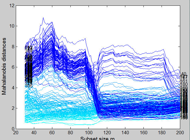
In the first part of the search, up to $m= 93$, the observations seem to fall into two groups. One has small distances and is composed of observations within or shortly to join the subset. Above these there are some outliers and then, higher still, a concentrated band of outliers, all of which are behaving similarly. When m=101 the search has reached a point at which at least one observation from Group 2 has to joint the subset. In fact, as the figure shows, due to the presence of outliers, this inclusion of units from both groups starts a little earlier. From $m=95$ the distances to the group of outliers decrease rapidly, as remote observations from Group 1, the genuine notes, join the subset. Around $m=105$ we can see that many of these former outliers are joining the subset (their distances decrease), while many of the units formerly in the subset leave (their distances increase). The crossing of two bands of outliers, seen here between $m=105$ and $m=115$, is typical of distances in a forward search when one multivariate normal distribution is fitted to data that contain two or more groups of appreciable size. Once the subset contains units from both groups, the search continues in a way similar and then identical to that of the earlier search. The right hand thirds of these two figures show identical patterns of Mahalanobis distances, the only difference being the vertical scale of the plots.

We now start with units in Group 2 (the forgeries).

load('swiss_banknotes');
Y=swiss_banknotes{:,:};
% start in the group of genuine notes
bs=101:120;
[out]=FSMeda(Y,bs,'init',30,'scaled',1);
malfwdplot(out);

The forward plot of scaled Mahalanobis distances  is broadly similar to that when we started with Group 1 (genuine notes), but the differences are informative. Before the interchange of units in the subset, the two groups seem more clearly separated than when we started from Group 1, although the non-fitted observations have a higher dispersion than before. The interchange starts earlier, because some units in Group 1 are closer to the centre of Group 2 than some of the outliers from Group 2. The distances for these outliers appear unaffected by the change in subset. The last third of the search is again the same as before.  

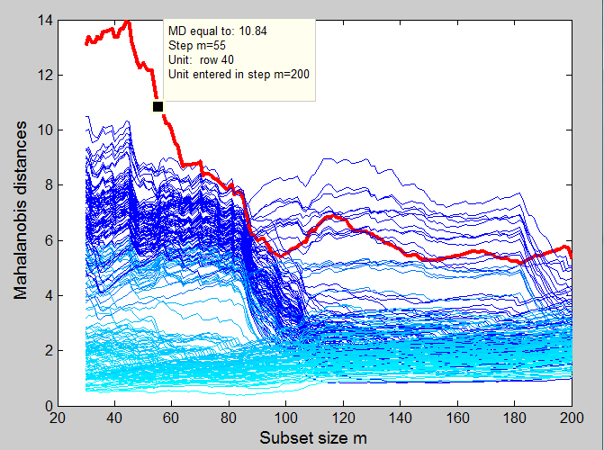
Finally we want to stress that with our personalized datatooltip clicking on a line it is possible to have a series of information about the selected trajectory (see yello box in the figure above).