Least trimmed squares (LTS) and Least median of squares (LMS)

The LTS regression estimators tries to find the estimate of $\beta$ which minimizes the sum of the $h$ smallest squared residuals, where $h$ must be at least half the number of observations.
The LMS regression estimators tries to find the estimate of $\beta$ which minimizes a quantile (generally the median) of squared residuals. LTS belongs to the class of L-estimators, so is asymptotically normal and has the usual convergence rate of $n^{-0.5}$. On the other hand, it is possible to show that even if the LMS estimator has an asymptotic normal distribution has a slower convergence rate of $n^{-1/3}$.

In the analysis which follows we analyze the transformed fidelity data and we compare the residuals which come out from the different options of traditional robust estimators (reweighted or not reweighted, individual tests or simultaneous tests confidence bands). In order to have a stable pattern of residuals we chose to extract 30000 subsets.

% Load the 'loyalty cards data' 
load('loyalty.txt');
% define y and X
y=loyalty(:,4);
X=loyalty(:,1:3);
% transform y
y1=y.^(0.4);

% Define nominal confidence level
conflev=0.99;
% Define number of subsets 
nsamp=30000;
% Define the main title of the plots
titl='';

% LMS with no rewighting
[outLMS]=LXS(y1,X,'nsamp',nsamp,'conflev',conflev);
h1=subplot(2,2,1);
laby='Scaled LMS residuals'; 
resindexplot(outLMS.residuals,'h',h1,'title',titl,'laby',laby,'numlab','','conflev',conflev)

% LTS with no rewighting
[outLTS]=LXS(y1,X,'nsamp',nsamp,'conflev',conflev,'lms',0);
h2=subplot(2,2,2);
laby='Scaled LTS residuals'; 
resindexplot(outLTS.residuals,'h',h2,'title',titl,'laby',laby,'numlab','','conflev',conflev);

% LMS with reweighting
[outLMSr]=LXS(y1,X,'nsamp',nsamp,'conflev',conflev,'rew',1);
h3=subplot(2,2,3);
laby='Scaled reweighted LMS residuals'; 
resindexplot(outLMSr.residuals,'h',h3,'title',titl,'laby',laby,'numlab','','conflev',conflev)

% LTS with reweighting
[outLTSr]=LXS(y1,X,'nsamp',nsamp,'conflev',conflev,'rew',1,'lms',0);
h4=subplot(2,2,4);
laby='Scaled reweighted LTS residuals'; 
resindexplot(outLTSr.residuals,'h',h4,'title',titl,'laby',laby,'numlab','','conflev',conflev);

The picture below gives the residuals which appear if we use LMS or LTS combined with the option reweighting and we use a nominal 99% confidence interval individual test. Notice that using standard individual test procedure with nominal size $\alpha$, in each dataset we expect to declare as outliers $\alpha\%$ of the values.

 

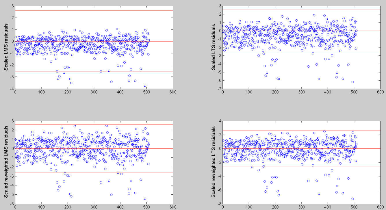
If we use a simultaneous confidence interval, that is if we specify conflev using the following code

conflev=1-0.01/length(y);

these are the plots that we get. Notice that using a simultaneous test procedure with size $\alpha$ we expect to find at least one outlier in $\alpha\%$ of the datasets.

 

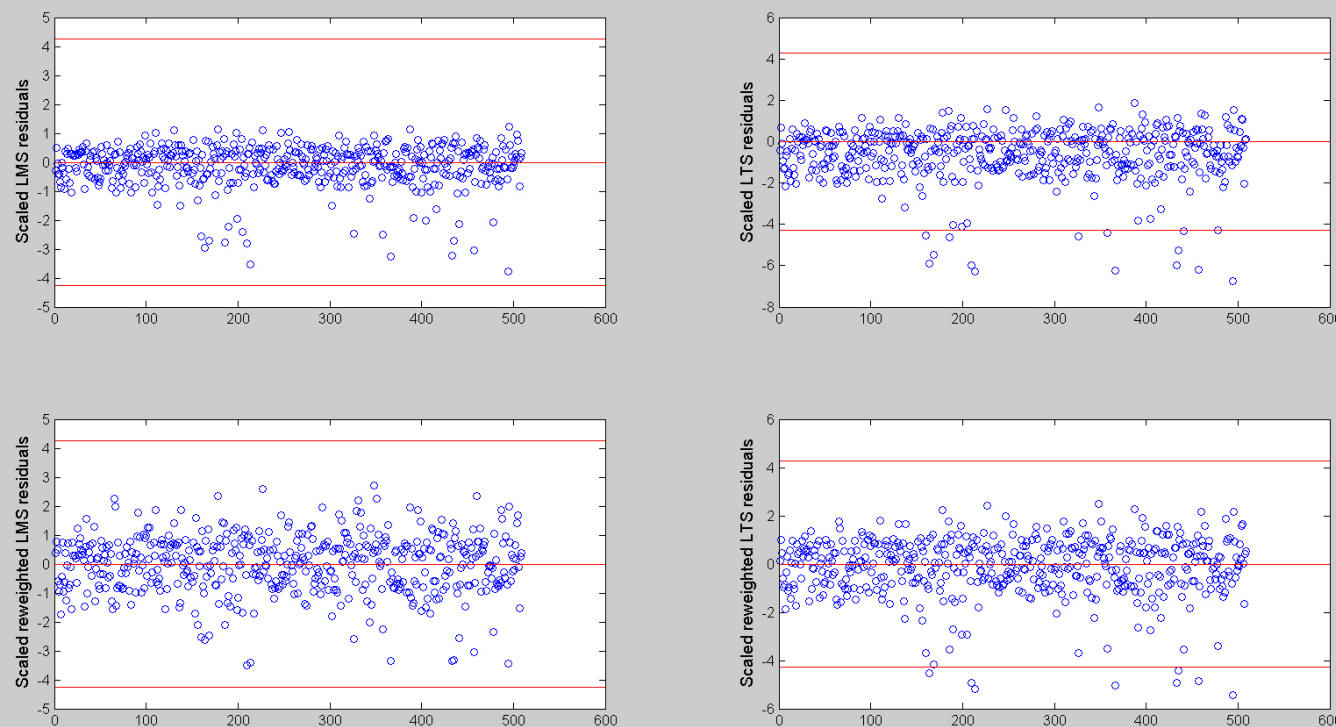
The structure of the residuals which comes from the use of LMS seems to be quite different from the one which comes out from LTS. If we use a simultaneous test procedure no unit is declared as outliers using LMS. The units declared as outliers in LTS depend on the fact that we use or not the option reweighting. In addition, it is not clear if the units declared as outliers form a group or which they exert on the fitted regression model.