S and MM estimators in linear regression

In the analysis which follows we analyze the transformed fidelity data and we compare the residuals which come out from the different options of traditional robust estimators (S and MM) using individual tests or simultaneous tests confidence bands. In order to have a stable pattern of residuals we chose to extract 30000 subsets.

% Load the 'loyalty cards data' 
load('loyalty.txt');
% define y and X
y=loyalty(:,4);
X=loyalty(:,1:3);
% transform y
y1=y.^(0.4);

% Define nominal confidence level
conflev=0.99;
% Define number of subsets 
nsamp=3000;
% Define the main title of the plots
titl='';

% S residuals
[outS]=Sreg(y1,X,'nsamp',nsamp,'conflev',conflev);
h1=subplot(2,1,1);
laby='Scaled S residuals'; 
resindexplot(outS.residuals,'h',h1,'title',titl,'laby',laby,'numlab','','conflev',conflev)


% MM scaled residuals
[outMM]=MMreg(y1,X,'Snsamp',nsamp,'conflev',conflev);
h3=subplot(2,1,2);
laby='Scaled MM residuals'; 
resindexplot(outMM.residuals,'h',h3,'title',titl,'laby',laby,'numlab','','conflev',conflev)

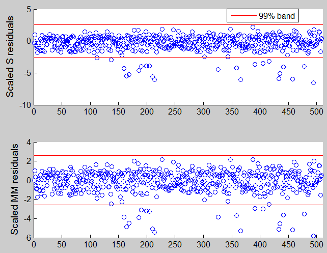
The picture below gives the residuals which appear if we use S or MM and we use a nominal 99% confidence interval individual test. Notice that using standard individual test procedure with nominal size $\alpha$, in each dataset we expect to declare as outliers $\alpha\%$ of the values.

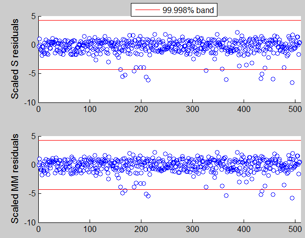
If we use a simultaneous confidence interval, that is if we specify conflev using the following code

conflev=1-0.01/length(y);

these are the plots that we get. Notice that using a simultaneous test procedure with size $\alpha$ we expect to find at least one outlier in $\alpha\%$ of the datasets.

 

The structure of the residuals which comes from the use of S estimators seems to be quite different from the one which comes out from MM estimators.