Documentation

Dynamic visualizazation in the candlestick plot

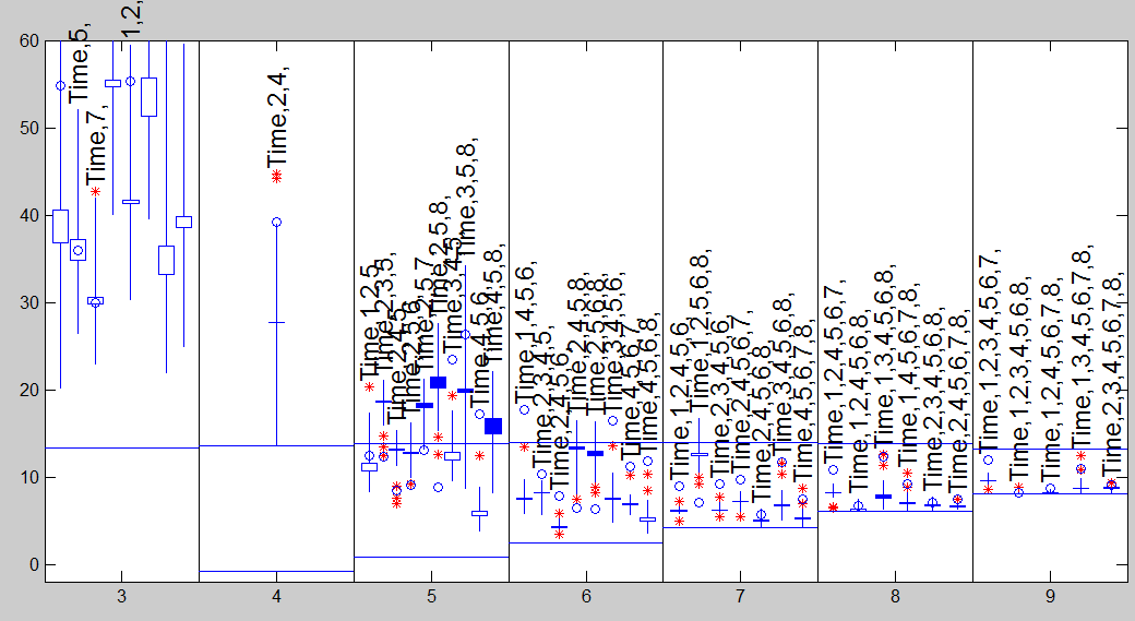
The generalized candlestick plot (Riani and Atkinson, 2010) is a plot which summarises the information on forward searches and model choice for numerous models. The detailed information about particular models can be extracted by brushing selected candles in the plot.

 

For example suppose that a candlestick plot has been built for the Ozone data using the following code.

    % Load Ozone data
    X=load('ozone.txt');
    % Tranform the response using logs
    X(:,end)=log(X(:,end));
    % Add a time trend
    X=[(-40:39)' X];
    % Define y
    y=X(:,end);
    % Define X
    X=X(:,1:end-1);
    labels={'Time','1','2','3','4','5','6','7','8'};
    % Robust model selection using Cp
    [Cpms]=FSRms(y,X,'labels',labels);
    % Candlestick plot
    cdsplot(Cpms);

The plot which is automatically displayed is as follows.

 

Using option 'cpbrush' inside function cdsplot it is possible to brush particular models with the mouse and to see immediately the corresponding trajectories of $C_p$ displayed in a new plot. 

 

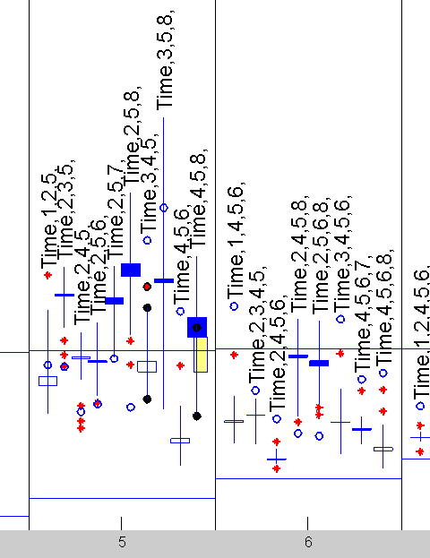
For example, suppose the user is interested to know more about models  Time345 and Time456, using the code

    cdsplot(Cpms,'cpbrush','1');

 

Once the required models are brushed with the mouse the selection appears in yellow color while the brushed candles are highlighted with black dots (see for an illustration figure below where model Time,4,5,8, has been selected):

 

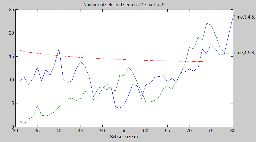
The plot of $C_p$ monitoring for the selected trajectories (in this case model Time,3,4,5) automatically appears in another window as shown in figure below.