FSMbonfbound
FSMbonfbound computes Bonferroni bounds for each step of the search (in mult analysis)
Description
Examples
 Example using default options.
Example using default options.
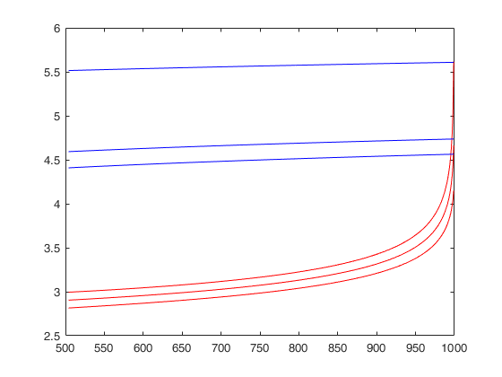
n=1000;
p=5;
init=floor(0.5*(n+p+1))+1;
MMDenv = FSMenvmmd(n,p,'init',init);
Bbound = FSMbonfbound(n,p,'init',init);
figure;
plot(MMDenv(:,1),MMDenv(:,2:end),'r',Bbound(:,1),Bbound(:,2:end),'b');
Related Examples
Input Arguments
Output Arguments
References
Atkinson, A.C. and Riani, M. (2006), Distribution theory and simulations for tests of outliers in regression, "Journal of Computational and Graphical Statistics", Vol. 15, pp. 460-476.