Heston2D
Heston2D simulates observations and instantaneous variances from the bivariate Heston model
Syntax
Description
Heston2D simulates, using the Euler–Maruyama method, observations and instantaneous variances from a 2-dimensional version of the model by [S. Heston, The Review of Financial Studies, Vol. 6, No. 2, 1993].
Example of call of Heston2D for obtaining process observations only.x
=Heston2D(T,
n,
parameters,
Rho,
x0,
V0)
Examples
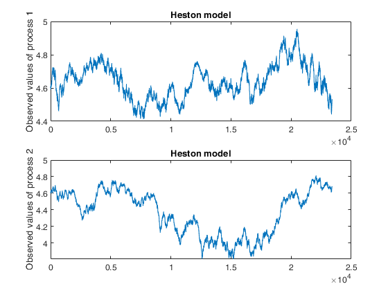
 Example of call of Heston2D for obtaining process observations only.
Example of call of Heston2D for obtaining process observations only.Generates observations from the bivariate Heston model.
T=1;
n=23400;
parameters=[0,0;0.4,0.4;2,2;1,1];
Rho=[0.5;-0.5;0;0;-0.5;0.5];
x0=[log(100),log(100)];
V0=[0.4,0.4];
x = Heston2D(T,n,parameters,Rho,x0,V0);
figure
subplot(2,1,1)
plot(x(:,1))
ylabel('Observed values of process 1')
title('Heston model')
subplot(2,1,2)
plot(x(:,2))
ylabel('Observed values of process 2')
title('Heston model')
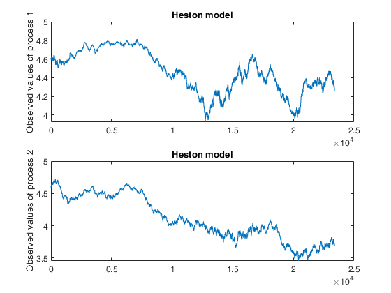
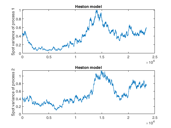
Example of call of Heston2D for obtaining process observations and volatility values.
Example of call of Heston2D for obtaining process observations and volatility values.Generates observations and volatilities from the bivariate Heston model.
T=1;
n=23400;
parameters=[0,0;0.4,0.4;2,2;1,1];
Rho=[0.5,-0.5,0,0,-0.5,0.5];
x0=[log(100),log(100)]; V0=[0.4,0.4];
[x,V] = Heston2D(T,n,parameters,Rho,x0,V0);
figure
subplot(2,1,1)
plot(x(:,1))
ylabel('Observed values of process 1')
title('Heston model')
subplot(2,1,2)
plot(x(:,2))
ylabel('Observed values of process 2')
title('Heston model')
figure
subplot(2,1,1)
plot(V(:,1))
ylabel('Spot variance of process 1')
title('Heston model')
subplot(2,1,2)
plot(V(:,2))
ylabel('Spot variance of process 2')
title('Heston model')

Example of call of Heston2D for obtaining process observations, volatility values and sampling times.
Example of call of Heston2D for obtaining process observations, volatility values and sampling times.Generates observations, volatilities and sampling times from the bivariate Heston model.
T=1;
n=23400;
parameters=[0,0;0.4,0.4;2,2;1,1];
Rho=[0.5,-0.5,0,0,-0.5,0.5];
x0=[log(100),log(100)]; V0=[0.4,0.4];
[x,V,t] = Heston2D(T,n,parameters,Rho,x0,V0);
figure
subplot(2,1,1)
plot(t,x(:,1))
xlabel('Time')
ylabel('Observed values of process 1')
title('Heston model')
subplot(2,1,2)
plot(t,x(:,2))
xlabel('Time')
ylabel('Observed values of process 2')
title('Heston model')
figure
subplot(2,1,1)
plot(t,V(:,1))
xlabel('Time')
ylabel('Spot variance of process 1')
title('Heston model')
subplot(2,1,2)
plot(t,V(:,2))
xlabel('Time')
ylabel('Spot variance of process 2')
title('Heston model')

Input Arguments
Output Arguments
More About
References
Heston, S. (1993), A closed-form solution for options with stochastic volatility with applications to bond and currency options, The Review of Financial Studies, Vol. 6, No. 2.