n x v data matrix; n observations and v variables. Rows of
Y represent observations, and columns represent variables.
Missing values (NaN's) and infinite values (Inf's) are
allowed, since observations (rows) with missing or infinite
values will automatically be excluded from the
computations.
Data Types: single|double
Specify optional comma-separated pairs of Name,Value arguments.
Name is the argument name and Value
is the corresponding value. Name must appear
inside single quotes (' ').
You can specify several name and value pair arguments in any order as
Name1,Value1,...,NameN,ValueN.
Example:
 'InitialEst',[]
, 'Snsamp',1000
, 'Sbdp',0.4
, 'Sbestr',10
, 'Sminsctol',1e-7
, 'Snsamp',1000
, 'Srefsteps',0
, 'Sreftol',1e-8
, 'Srefstepsbestr',10
, 'Sreftolbestr',1e-10
, 'eff',0.99
, 'effshape',1
, 'refsteps',10
, 'tol',1e-10
, 'conflev',0.99
, 'plots',0
, 'nocheck',1
, 'ysave',1
InitialEst must contain the following fields:
| Value |
Description |
loc0 |
1 x v vector (estimate of the centroid)
|
shape0 |
v x v matrix (estimate of the shape matrix)
|
auxscale |
scalar (estimate of the scale parameter).
If InitialEst is empty (default)
program uses S estimators. In this last case it is
possible to specify the options given in function Smult.
|
Example: 'InitialEst',[]
Data Types: struct
.
See function Smult for more details on these options.
It is necessary to add to the S options the letter
S at the beginning. For example, if you want to use the
optimal rho function the supplied option is
'Srhofunc','optimal'. For example, if you want to use 3000
subsets, the supplied option is 'Snsamp',3000
Example: 'Snsamp',1000
Data Types: single | double
It measures the fraction of outliers
the algorithm should resist. In this case any value greater
than 0 but smaller or equal than 0.5 will do fine (default=0.5).
Note that given bdp nominal
efficiency is automatically determined.
Example: 'Sbdp',0.4
Data Types: double
Scalar
defining number of "best betas" to remember from the
subsamples. These will be later iterated until convergence
(default=5)
Example: 'Sbestr',10
Data Types: single | double
Value of tolerance for the iterative
procedure for finding the minimum value of the scale
for each subset and each of the best subsets
(It is used by subroutine minscale.m)
The default value is 1e-7;
Example: 'Sminsctol',1e-7
Data Types: single | double
If nsamp=0 all subsets will be extracted.
They will be (n choose p).
If the number of all possible subset is <1000 the
default is to extract all subsets otherwise just 1000.
Example: 'Snsamp',1000
Data Types: single | double
Number of refining
iterationsin each subsample (default = 3).
refsteps = 0 means "raw-subsampling" without iterations.
Example: 'Srefsteps',0
Data Types: single | double
The default value is 1e-6;
Example: 'Sreftol',1e-8
Data Types: single | double
Scalar defining number of refining iterations for each
best subset (default = 50).
Example: 'Srefstepsbestr',10
Data Types: single | double
Tolerance for the refining steps
for each of the best subsets
The default value is 1e-8;
Example: 'Sreftolbestr',1e-10
Data Types: single | double
Scalar defining nominal efficiency (i.e. a number between
0.5 and 0.99). The default value is 0.95
Asymptotic nominal efficiency is:
Example: 'eff',0.99
Data Types: double
If effshape=1 efficiency refers to shape
efficiency else (default) efficiency refers to location
Example: 'effshape',1
Data Types: double
Scalar defining maximum number of iterations in the MM
loop. Default value is 100.
Example: 'refsteps',10
Data Types: double
Scalar controlling tolerance in the MM loop.
Default value is 1e-7
Example: 'tol',1e-10
Data Types: double
Usually conflev=0.95, 0.975 0.99 (individual alpha)
or 1-0.05/n, 1-0.025/n, 1-0.01/n (simultaneous alpha).
Default value is 0.975
Example: 'conflev',0.99
Data Types: double
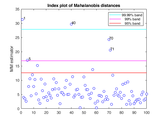
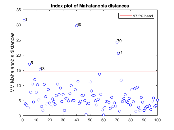
If plots is a structure or scalar equal to 1, generates:
(1) a plot of Mahalanobis distances against index number. The
confidence level used to draw the confidence bands for
the MD is given by the input option conflev. If conflev is
not specified a nominal 0.975 confidence interval will be
used.
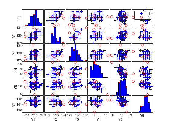
(2) a scatter plot matrix with the outliers highlighted.
If plots is a structure it may contain the following fields
| Value |
Description |
labeladd |
if this option is '1', the outliers in the
spm are labelled with their unit row index. The
default value is labeladd='', i.e. no label is
added.
|
nameY |
cell array of strings containing the labels of
the variables. As default value, the labels which
are added are Y1, ...Yv.
|
Example: 'plots',0
Data Types: single | double
If nocheck is equal to 1
no check is performed on
matrix Y. As default nocheck=0.
Example: 'nocheck',1
Data Types: double
Scalar that is set to 1 to request that the data matrix Y
is saved into the output structure out. This feature is
meant at simplifying the use of function malindexplot.
Default is 0, i.e. no saving is done.
Example: 'ysave',1
Data Types: double
 MMmult with all default options.