biplotFS
biplotFS calls biplotAPP.mlapp to show a dynamic biplot.
Description
The svd of $Z=zscore(Y)$ \[ Z= U \Gamma^* V^T \] and its best rank two approximation \[ Z \approx U_{(2)} \Gamma_{(2)}^* V_{(2)}^T \]
where $U_{(2)}$ is $n \times 2$ matrix (first two columns of $U$) and $V_{(2)}$ is $p \times 2$ (first two columns of matrix $V$, $\Gamma_{(2)}^*$ is a $2 \times 2$ diagonal matrix, which contains the first two largest singular values of matrix $Z$ (square root of the eigenvalues of matrix $Z^TZ=(n-1)R$) where $R$ is the correlation matrix.
We can also write
\[ \frac{Z}{\sqrt{n-1}} \approx U_{(2)}\frac{\Gamma_{(2)}^*}{\sqrt{n-1}} V_{(2)}^T \] \[ Z \approx \sqrt{n-1} U_{(2)}\frac{\Gamma_{(2)}^*}{\sqrt{n-1}} V_{(2)}^T \] \[ Z \approx \sqrt{n-1} U_{(2)} \Gamma_{(2)} V_{(2)}^T \]where $\Gamma_{(2)} = \Gamma_{(2)}^*/ \sqrt{n-1}$.
In this way $\Gamma_{(2)}$ contains the singular values (square root of the eigenvalues) of matrix $Z^TZ/(n-1)=R$ (correlation matrix).
The last equation can be written as function of two parameters $\alpha \in [0 1]$ and $\omega \in [0 1]$
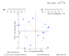
\[ Z \approx \left[ (\sqrt{n-1})^\omega U_{(2)} \Gamma_{(2)}^\alpha \right] [ \Gamma_{(2)}^{1-\alpha} V_{(2)}^T (\sqrt{n-1})^{1-\omega} ] \]In the dynamic biplot the $n$ row points are represented by $n \times 2$ matrix:
\[ \left[ (\sqrt{n-1})^\omega U_{(2)} \Gamma_{(2)}^\alpha \right] \] and the $p$ column points (arrows) through $2 \times p$ matrix \[ [ \Gamma_{(2)}^{1-\alpha} V_{(2)}^T (\sqrt{n-1})^{1-\omega} ] \] Note that if $\omega=1$ and $\alpha=0$ row points are \[ \sqrt{n-1} U_{(2)}= Z V_{(2)} \Gamma_{(2)}^{-1} \]
that is, row points are the standardized principal components scores.
\[ cov (\sqrt{n-1} U_{(2)}) = I_2= \left( \begin{array}{cc} 1 & 0 \\ 0 & 1 \\ \end{array} \right) \] Column points are \[ \Gamma_{(2)} V_{(2)}^T \]
that is, the arrows are associated with the correlations between the variables and the first two principal components.
The length of the arrow is exactly equal to the communality of the associated variable.
In this case, the unit circle is also shown on the screen and option axis equal is set.
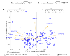
On the other hand, if $\omega=1$ and $\alpha=1$ the $n$ rows of $Z$ (of dimension $n \times p$) can be represented using $n \times 2$ matrix:
\[ \sqrt{n-1} U_{(2)} \Gamma_{(2)} = Z V_{(2)} \] In this case, the row points are the (non normalized) scores, that is \[ cov(\sqrt{n-1} U_{(2)} \Gamma_{(2)}) =cov( Z V_{(2)})= \left( \begin{array}{cc} \lambda_1 & 0 \\ 0 & \lambda_2 \\ \end{array} \right) \] With this parametrization the column points (arrows) are nothing but the coordinates of the first two eigenvectors \[ V_{(2)}^T \]
Also in this case, the unit circle is given and option axis equal is set.
In general if $\omega$ decreases, the length of the arrows increases and the coordinates of row points are squeezed towards the origin.
In the app it is also possible to color row points depending on the orthogonal distance ($OD_i$) of each observation to the PCA subspace.
For example, if the subspace is defined by the first two principal components, $OD_i$ is computed as:
\[ OD_i=|| z_i- V_{(2)} V_{(2)}' z_i || \] If an optional input argument, bsb or bdp, is specified, it is possible to have in the app two tabs that enable the user to select the breakdown point of the analysis of the subset size to use in the svd. The units that are declared as outliers or the units outside the subset are shown in the plot with filled circles.
biplotFS(
use of biplotFS on the dataset referred to Italian cities.Y,
Name, Value)
Examples
 use of biplotFS on the ingredients dataset.
use of biplotFS on the ingredients dataset.
load hald
% Operate on the correlation matrix (default).
% Use standardized principal components (for row points) and
% correlation between variables and principal components (for column
% points, arrows).
close all
biplotFS(ingredients,'omega',1,'alpha',0);
When \omega=1 and \alpha=0
Row points represent standardized principal components sqrt(n-1)*U=ZV*\Gamma^-1
Arrows represent correlations between variables and principal components \Gamma*V
The length of the arrows is the communality of the variable
In this case the unit circle is also shown
When \omega=1 and \alpha=0
Row points represent standardized principal components sqrt(n-1)*U=ZV*\Gamma^-1
Arrows represent correlations between variables and principal components \Gamma*V
The length of the arrows is the communality of the variable
In this case the unit circle is also shown