ctlcurves
ctlcurves computes Classification Trimmed Likelihood Curves
Description
ctlcurves applies tclust several times on a given dataset while parameters alpha and k are altered. The resulting object gives an idea of the optimal trimming level and number of clusters considering a particular dataset.
Example of the use of options alpha, kk and bands.out
=ctlcurves(Y,
Name, Value)
Examples
 Example of use of ctlcurves with all default options.
Example of use of ctlcurves with all default options.Load the geyser data
rng('default')
rng(10)
Y=load('geyser2.txt');
% Just use a very small sumber of subsets for speed reasons.
nsamp=10;
out=ctlcurves(Y,'nsamp',nsamp);
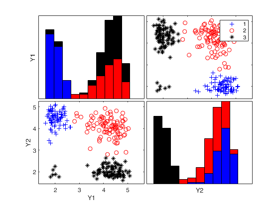
% Show the automatic classification
spmplot(Y,out.LRToptimalIDX(:,1));
k=1
k=2
k=3
k=4
k=5
Bands k=1
Bands k=2
Bands k=3
Bands k=4
Bands k=5
Example of the use of options alpha, kk and bands.
Personalized levels of trimming.
alpha=0:0.05:0.15;
% bands is passed as a false boolean. No bands are shown.
bands=false;
Y=load('geyser2.txt');
% Just use a very small sumber of subsets for speed reasons.
rng(100)
nsamp=10;
out=ctlcurves(Y,'alpha',alpha,'kk',2:4,'bands',bands,'nsamp',nsamp);
Related Examples
option bands passed as struct.
option bands passed as struct.load the M5 data.
Y=load('M5data.txt');
Y=Y(:,1:2);
bands=struct;
% just 20 simulations to construct the bands.
bands.nsimul=20;
% Exclude the units detected as outliers for each group.
bands.valSolution=true;
% One of the extracted subsets is based on solutions found with real data
bands.usepriorSol=true;
% Just use a very small sumber of subsets for speed reasons.
nsamp=20;
rng(100)
out=ctlcurves(Y,'bands',bands,'kk',2:4,'alpha',0:0.02:0.1,'nsamp',nsamp);
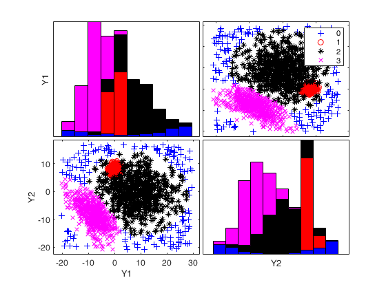
% Show final classification using intersection of confidence bands.
spmplot(Y,out.CTLoptimalIDX);
k=2
k=3
k=4
Bands k=2
Bands k=3
Bands k=4
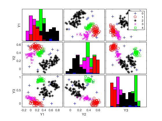
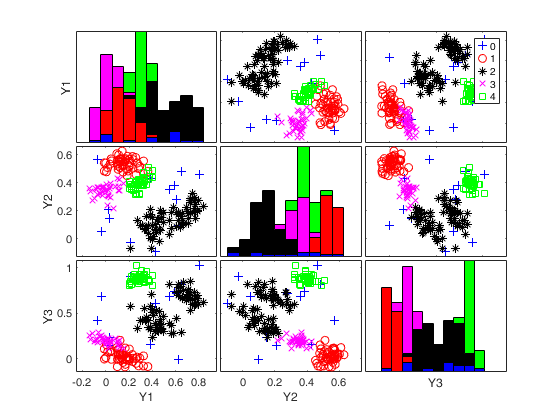
An example with many groups.
An example with many groups.Simulate data with 5 groups in 3 dimensions
rng(1)
k=5; v=3;
n=200;
Y = MixSim(k, v, 'MaxOmega',0.01);
[Y]=simdataset(n, Y.Pi, Y.Mu, Y.S, 'noiseunits', 10);
% Just use a very small sumber of subsets for speed reasons.
nsamp=5;
out=ctlcurves(Y,'plots',0,'kk',4:6,'nsamp',nsamp);
spmplot(Y,out.CTLoptimalIDX);
k=4
k=5
k=6
Bands k=4
Bands k=5
Bands k=6
Input Arguments
Y — Input data.
Matrix.
Data matrix containing n observations on v variables, Rows of Y represent observations, and columns represent variables. Observations (rows) with missing (NaN) or or infinite (Inf) values will automatically be excluded from the computations.
Data Types: double
Name-Value Pair Arguments
Specify optional comma-separated pairs of Name,Value arguments.
Name is the argument name and Value
is the corresponding value. Name must appear
inside single quotes (' ').
You can specify several name and value pair arguments in any order as
Name1,Value1,...,NameN,ValueN.
 'alpha',[0 0.05 0.1]
, 'bands',true
, 'kk',1:4
, 'cshape',10
, 'equalweights',true
, 'msg',false
, 'mixt',1
, 'nocheck',10
, 'nsamp',1000
, 'refsteps',10
, 'reftol',1e-05
, 'restrfactor',12
, 'restrtype','deter'
, 'startv1',1
, 'cleanpool',1
, 'numpool',4
, 'plots',1
, 'Ysave',false
alpha
—trimming level to monitor.vector.
Vector which specifies the values of trimming levels which have to be considered.
For example if alpha=[0 0.05 0.1] ctlcurves considers these 3 values of trimming level.
The default for alpha is vector 0:0.02:0.10;
Example: 'alpha',[0 0.05 0.1]
Data Types: double
bands
—confidence bands for the curves.boolean | struct.
If bands is a scalar boolean equal to true (default), 50 per cent confidence bands are computed (and are shown on the screen if plots=1), likelihood ratio tests are also computed and the solutions found by these two methods are given. If bands is a scalar boolean equal to false, bands and likelihood ratio tests are not computed.
If bands is a struct bands are computed and the structure may contain the following fields:
| Value | Description |
|---|---|
conflev |
scalar in the interval (0 1) which contains the confidence level of the bands (default is 0.5). |
nsamp |
Number of subsamples to extract in the bootstrap replicates. If this field is not present and or it is empty the number of subsamples which is used in the bootstrap replicates is equal to the one used for real data (input option nsamp). |
nsimul |
number of replicates to use to create the confidence bands and likelihood ratio tests. The default value of bands.nsimul is 60 in order to provide the output in a reasonal time. Note that for stable results we recommentd a value of bands.nsimul equal to 100. |
valSolution |
boolean which specifies if it is necessary to perform an outlier detection procedure on the components which have been found using optimalK and optimal alpha. If bands.valSolution is true then units detected as outliers in each component are assigned to the noise group. If bands.valSolution is false (default) or it is not present nothing is done. |
usepriorSol |
Initialization of the EM for a particular subset. boolean. If bands.usepriorSol is true, we initialize the EM algorithm for one of the bands.nsamp subsets with the solution which has been found with real data, else if it is false (default) no prior information is used in any of the extracted subsets. |
outliersFromUniform |
way of generating the outliers in the bootstrap replicates. Boolean. If outliersFromUniform is true (default) the outliers are generated using the uniform distribution in such a way that their squared Mahalanobis distance from the centroids of each existing group is larger then the quantile 1-0.999 of the Chi^2 distribution with p degrees of freedom. For additional details see input option noiseunits of simdataset. If outliersFromUniform is false the outliers are the units which have been trimmed after applying tclust for the particular combination of values of k and alpha. |
nsimulExtra |
number of replicates to use to compute the empirical pvalue of LRtest if multiple solutions are found given a value of alpha (default is 50). |
nsampExtra |
number of subsamples to extract in each replicate to compute the empirical pvalue of LRtest if multiple solutions are found given a value of alpha (default is 2000). |
usepriorSolExtra |
Initialization of the EM for particular subset. boolean. If bands.usepriorSolExtra is true, we initialize the EM algorithm for one of the bands.nsampExtra subsets with the solution which has been found with real data, else if it is false (default) no prior information is used in any of the extracted subsets. |
crit |
scalar which defines the empirical p-value which is used to define a solution as significant and to reject the null hypotesis of smaller groups in the likelihood ratio test. The default value of crit is 0.02, that is when we test against k+1 given a certain value of \alpha, if the empirical p-value is greater than crit we accept the null hypothesis of k groups. |
Example: 'bands',true
Data Types: logical | struct
kk
—number of mixture components.integer vector.
Integer vector specifying the number of mixture components (clusters) for which trimmed likelihoods are calculated.
Vector. The default value of kk is 1:5.
Example: 'kk',1:4
Data Types: int16 | int32 | single | double
cshape
—constraint to apply to each of the shape matrices.scalar greater | equal than 1.
This options only works is 'restrtype' is 'deter'.
When restrtype is deter the default value of the "shape" constraint (as defined below) applied to each group is fixed to c_{shape}=10^{10}, to ensure the procedure is (virtually) affine equivariant. In other words, the decomposition or the j-th scatter matrix \Sigma_j is
\Sigma_j=\lambda_j^{1/v} \Omega_j \Gamma_j \Omega_j' where \Omega_j is an orthogonal matrix of eigenvectors, \Gamma_j is a diagonal matrix with |\Gamma_j|=1 and with elements \{\gamma_{j1},...,\gamma_{jv}\} in its diagonal (proportional to the eigenvalues of the \Sigma_j matrix) and |\Sigma_j|=\lambda_j. The \Gamma_j matrices are commonly known as "shape" matrices, because they determine the shape of the fitted cluster components. The following k constraints are then imposed on the shape matrices: \frac{\max_{l=1,...,v} \gamma_{jl}}{\min_{l=1,...,v} \gamma_{jl}}\leq c_{shape}, \text{ for } j=1,...,k,In particular, if we are ideally searching for spherical clusters it is necessary to set c_{shape}=1. Models with variable volume and spherical clusters are handled with 'restrtype' 'deter', 1<restrfactor<\infty and cshape=1.
The restrfactor=cshape=1 case yields a very constrained parametrization because it implies spherical clusters with equal volumes.
Example: 'cshape',10
Data Types: single | double
equalweights
—cluster weights in the concentration and assignment steps.logical.
A logical value specifying whether cluster weights shall be considered in the concentration, assignment steps and computation of the likelihood.
Example: 'equalweights',true
Data Types: Logical
msg
—Message on the screen.boolean.
Boolean which controls whether to display or not messages about code execution.
Example: 'msg',false
Data Types: logical
mixt
—Mixture modelling or crisp assignment.scalar.
Option mixt specifies whether mixture modelling or crisp assignment approach to model based clustering must be used.
In the case of mixture modelling parameter mixt also controls which is the criterion to find the untrimmed units in each step of the maximization.
If mixt >=1 mixture modelling is assumed else crisp assignment. The default value is mixt=0 (i.e. crisp assignment).
In mixture modelling the likelihood is given by:
\prod_{i=1}^n \sum_{j=1}^k \pi_j \phi (y_i; \; \theta_j), while in crisp assignment the likelihood is given by: \prod_{j=1}^k \prod _{i\in R_j} \phi (y_i; \; \theta_j),where R_j contains the indexes of the observations which are assigned to group j.
Remark - if mixt>=1 previous parameter equalweights is automatically set to 1.
Parameter mixt also controls the criterion to select the units to trim, if mixt = 2 the h units are those which give the largest contribution to the likelihood that is the h largest values of:
\sum_{j=1}^k \pi_j \phi (y_i; \; \theta_j) \qquad i=1, 2, ..., n, else if mixt=1 the criterion to select the h units is exactly the same as the one which is used in crisp assignment. That is: the n units are allocated to a cluster according to criterion: \max_{j=1, \ldots, k} \hat \pi'_j \phi (y_i; \; \hat \theta_j)and then these n numbers are ordered and the units associated with the largest h numbers are untrimmed.
Example: 'mixt',1
Data Types: single | double
nocheck
—Check input arguments.scalar.
If nocheck is equal to 1 no check is performed on matrix Y. As default nocheck=0.
Example: 'nocheck',10
Data Types: single | double
nsamp
—number of subsamples to extract.scalar | matrix.
If nsamp is a scalar it contains the number of subsamples which will be extracted. If nsamp=0 all subsets will be extracted.
Remark - if the number of all possible subset is <300 the default is to extract all subsets, otherwise just 300.
- If nsamp is a matrix it contains in the rows the indexes of the subsets which have to be extracted. nsamp in this case can be conveniently generated by function subsets.
nsamp can have k columns or k*(v+1) columns. If nsamp has k columns the k initial centroids each iteration i are given by X(nsamp(i,:),:) and the covariance matrices are equal to the identity.
- If nsamp has k*(v+1) columns the initial centroids and covariance matrices in iteration i are computed as follows X1=X(nsamp(i,:),:) mean(X1(1:v+1,:)) contains the initial centroid for group 1 cov(X1(1:v+1,:)) contains the initial cov matrix for group 1 1 mean(X1(v+2:2*v+2,:)) contains the initial centroid for group 2 cov((v+2:2*v+2,:)) contains the initial cov matrix for group 2 1 ...
mean(X1((k-1)*v+1:k*(v+1))) contains the initial centroids for group k cov(X1((k-1)*v+1:k*(v+1))) contains the initial cov matrix for group k REMARK - if nsamp is not a scalar option option below startv1 is ignored. More precisely if nsamp has k columns startv1=0 elseif nsamp has k*(v+1) columns option startv1=1.
Example: 'nsamp',1000
Data Types: double
refsteps
—Number of refining iterations.scalar.
Number of refining iterations in subsample. Default is 15. refsteps = 0 means "raw-subsampling" without iterations.
Example: 'refsteps',10
Data Types: single | double
reftol
—scalar.default value of tolerance for the refining steps.
The default value is 1e-14;
Example: 'reftol',1e-05
Data Types: single | double
restrfactor
—Restriction factor.scalar.
Positive scalar which constrains the allowed differences among group scatters. Larger values imply larger differences of group scatters. On the other hand a value of 1 specifies the strongest restriction forcing all eigenvalues/determinants to be equal and so the method looks for similarly scattered (respectively spherical) clusters. The default is to apply restrfactor to eigenvalues. In order to apply restrfactor to determinants it is is necessary to use optional input argument cshape.
Example: 'restrfactor',12
Data Types: double
restrtype
—type of restriction.character.
The type of restriction to be applied on the cluster scatter matrices. Valid values are 'eigen' (default), or 'deter'.
eigen implies restriction on the eigenvalues while deter implies restriction on the determinants. If restrtype is 'deter' it is possible to control the constraints on the shape matrices using optional input argument cshape.
Example: 'restrtype','deter'
Data Types: char
startv1
—how to initialize centroids and cov matrices.scalar.
If startv1 is 1 then initial centroids and and covariance matrices are based on (v+1) observations randomly chosen, else each centroid is initialized taking a random row of input data matrix and covariance matrices are initialized with identity matrices.
Remark 1- in order to start with a routine which is in the required parameter space, eigenvalue restrictions are immediately applied. The default value of startv1 is 1.
Remark 2 - option startv1 is used just if nsamp is a scalar (see for more details the help associated with nsamp).
Example: 'startv1',1
Data Types: single | double
cleanpool
—clean pool.scalar.
cleanpool is 1 if the parallel pool has to be cleaned after the execution of the routine. Otherwise it is 0. The default value of cleanpool is 0. Clearly this option has an effect just if previous option numpool is >
1.
Example: 'cleanpool',1
Data Types: single | double
numpool
—number of pools for parellel computing.scalar.
If numpool > 1, the routine automatically checks if the Parallel Computing Toolbox is installed and distributes the random starts over numpool parallel processes. If numpool <= 1, the random starts are run sequentially. By default, numpool is set equal to the number of physical cores available in the CPU (this choice may be inconvenient if other applications are running concurrently). The same happens if the numpool value chosen by the user exceeds the available number of cores.
REMARK 1: Unless you adjust the cluster profile, the default maximum number of workers is the same as the number of computational (physical) cores on the machine.
REMARK 2: In modern computers the number of logical cores is larger than the number of physical cores. By default, MATLAB is not using all logical cores because, normally, hyper-threading is enabled and some cores are reserved to this feature.
REMARK 3: It is because of Remarks 3 that we have chosen as default value for numpool the number of physical cores rather than the number of logical ones. The user can increase the number of parallel pool workers allocated to the multiple start monitoring by: - setting the NumWorkers option in the local cluster profile settings to the number of logical cores (Remark 2). To do so go on the menu "Home|Parallel|Manage Cluster Profile" and set the desired "Number of workers to start on your local machine".
- setting numpool to the desired number of workers;
Therefore, *if a parallel pool is not already open*, UserOption numpool (if set) overwrites the number of workers set in the local/current profile. Similarly, the number of workers in the local/current profile overwrites default value of 'numpool' obtained as feature('numCores') (i.e. the number of physical cores).
Example: 'numpool',4
Data Types: double
plots
—Plot on the screen.scalar.
If plots = 1, a plot of the CTLcurves is shown on the screen. If input option bands is not empty confidence bands are also shown.
Example: 'plots',1
Data Types: single | double
Ysave
—save input matrix.boolean.
Boolan that is set to true to request that the input matrix Y is saved into the output structure out. Default is 1, that is matrix Y is saved inside output structure out.
Example: 'Ysave',false
Data Types: logical
Output Arguments
out — description
Structure
Structure which contains the following fields:
| Value | Description |
|---|---|
Mu |
cell of size length(kk)-by-length(alpha) containing the estimate of the centroids for each value of k and each value of alpha. More precisely, suppose kk=1:4 and alpha=[0 0.05 0.1], out.Mu{2,3} is a matrix with two rows and v columns containing the estimates of the centroids obtained when alpha=0.1. |
Sigma |
cell of size length(kk)-by-length(alpha) containing the estimate of the covariance matrices for each value of k and each value of alpha. More precisely, suppose kk=1:4 and alpha=[0 0.05 0.1], out.Sigma{2,3} is a 3D array of size v-by-v-by-2 containing the estimates of the covariance matrices obtained when alpha=0.1. |
Pi |
cell of size length(kk)-by-length(alpha) containing the estimate of the group proportions for each value of k and each value of alpha. More precisely, suppose kk=1:4 and alpha=[0 0.05 0.1], out.Pi{2,3} is a 3D array of size v-by-v-by-2 containing the estimates of the covariance matrices obtained when alpha=0.1. |
IDX |
cell of size length(kk)-by-length(alpha) containing the final assignment for each value of k and each value of alpha. More precisely, suppose kk=1:4 and alpha=[0 0.05 0.1], out.IDX{2,3} is a vector of length(n) containing the containinig the assignment of each unit obtained when alpha=0.1. Elements equal to zero denote unassigned units. |
CTL |
matrix of size length(kk)-by-length(alpha) containing the values of the trimmed likelihood curves for each value of k and each value of alpha. This output (and all the other output below which start with CTL) are present only if input option bands is true or is a struct. All the other fields belo |
CTLbands |
3D array of size length(kk)-by-length(alpha)-by-nsimul containing the nsimul replicates of out.CTL. |
CTLlikLB |
matrix of size length(kk)-by-length(alpha) containing the lower confidence bands of the trimmed likelihood curves for each value of k and each value of alpha. |
CTLlikUB |
matrix of size length(kk)-by-length(alpha) containing the upper confidence bands of the trimmed likelihood curves for each value of k and each value of alpha. T |
CTLlik050 |
matrix of size length(kk)-by-length(alpha) containing the central confidence bands of the trimmed likelihood curves for each value of k and each value of alpha. |
CTLtentSol |
matrix with size m-by-4. Details of the ordered solutions where there was intersection between two consecutive trimmed likelihood curves. First column contains the value of k, second column the value of alpha, third column the index associated to the best value of alpha, fourth colum index associated with the best value of kk. |
CTLoptimalAlpha |
scalar, optimal value of trimming. |
CTLoptimalK |
scalar, optimal number of clusters, stored as a positive integer value. |
CTLoptimalIDX |
n-by-1 vector containing assignment of each unit to each of the k groups in correspodence of OptimalAlpha and OptimalK. Cluster names are integer numbers from 1 to k. 0 indicates trimmed observations. The fields which follow which start with LRT refer to the likilhood ratio test |
LRTpval |
table with size length(kk)-1-times-length(alpha) which stores the relative frequency in which the Likelihood ratio test is greater than the corresponding bootstrap test. as a positive integer value. |
LRTtentSol |
matrix with size m-by-8. Details of the ordered solutions using the likelihood ratio test. First column (index): the index number of the solution. Second column (k): the value of k. Third column (alpha): the value of alpha. Fourth column (Truesol) contains 1 if the p-value beyond the threshold is always above k shown in the second column for all k^* >k else it contains 0. Fifth and sixth columns (kindex and alphaindex) contain the index numbers of optimal input values kk and alpha. Seventh column (kbestGivenalpha) contains 1 in correspondence of the best solution for each value of k (given alpha). Eight column (ProperSize) contains 1 if the solution which has been found has a minimum group size which is greater than n*max(alpha). |
LRTtentSolt |
table with the same size of LRTtentSol containing the same information of array out.TentSolLR in table format. |
LRTtentSolIDX |
matrix with size n-by-size(out.LRTtentSol,1) with the allocation associated with the tentative solutions found in out.LRTtentSol. First column refers to solution in row 1 of out.LRTtentSol ... |
LRToptimalAlpha |
scalar, optimal value of trimming. |
LRToptimalK |
scalar, optimal number of clusters, stored as a positive integer value. |
LRToptimalIDX |
n-by-r vector containing assignment of each unit to each of the k groups in correspondence of OptimalAlpha and OptimalK. Cluster names are integer numbers from 1 to k. 0 indicates trimmed observations. The fields which follow which start with LRT refer to the likelihood ratio test. |
kk |
vector containing the values of k (number of components) which have been considered. This vector is equal to input optional argument kk if kk had been specified else it is equal to 1:5. |
alpha |
vector containing the values of the trimming level which have been considered. This vector is equal to input optional argument alpha. |
tclustPAR |
a structure containing all the parameters used by tclust (restrfactor, mixt, restrtype. refsteps, equalweights, reftol, cshape, nsamp, nsampExtra, outliersFromUniform, nsimulExtra and usepriorSolExtra). |
Y |
Original data matrix Y. The field is present if option Ysave is set to 1. |
More About
Additional Details
These curves show the values of the trimmed classification (log)-likelihoods when altering the trimming proportion alpha and the number of clusters k. The careful examination of these curves provides valuable information for choosing these parameters in a clustering problem. For instance, an appropriate k to be chosen is one that we do not observe a clear increase in the trimmed classification likelihood curve for k with respect to the k+1 curve for almost all the range of alpha values. Moreover, an appropriate choice of parameter alpha may be derived by determining where an initial fast increase of the trimmed classification likelihood curve stops for the final chosen k (Garcia Escudero et al. 2011). This routine adds confidence bands in order to provide an automatic criterion in order to choose k and alpha. Optimal trimming level is chosen as the smallest value of alpha such that the bands for two consecutive values of k intersect and computes a bootstrap test for two consecutive values of k given alpha.
References
Garcia-Escudero, L.A., Gordaliza, A., Matran, C. and Mayo-Iscar A., (2011), "Exploring the number of groups in robust model-based clustering." Statistics and Computing, Vol. 21, pp. 585-599.