
|
makecontentsfileFS |
malindexplot |
 |
malfwdplot
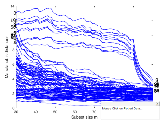
malfwdplot plots the trajectories of scaled Mahalanobis distances along the search
Description
Examples
 Produce monitoring MD plot with all the default options.
Produce monitoring MD plot with all the default options.Generate input structure for malfwdplot
n=100;
p=4;
state1=141243498;
randn('state', state1);
Y=randn(n,p);
kk=[1:10];
Y(kk,:)=Y(kk,:)+4;
[fre]=unibiv(Y);
m0=20;
bs=fre(1:m0,1);
[out]=FSMeda(Y,bs,'plots',1,'init',30);
% Produce monitoring MD plot with all the default options
malfwdplot(out)
Warning: Using 'state' to set RANDN's internal state causes RAND, RANDI, and
RANDN to use legacy random number generators.  This syntax is not recommended.
See <a href="matlab:helpview([docroot '\techdoc\math\math.map'],'update_random_number_generator')">Replace Discouraged Syntaxes of rand and randn</a> to use RNG to replace the
old syntax.

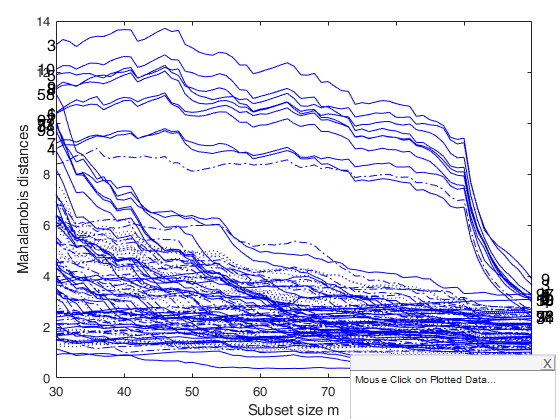
Example of the use of some options inside structure standard.
Example of the use of some options inside structure standard.
n=100;
p=4;
state1=141243498;
randn('state', state1);
Y=randn(n,p);
kk=[1:10];
Y(kk,:)=Y(kk,:)+4;
[fre]=unibiv(Y);
m0=20;
bs=fre(1:m0,1);
[out]=FSMeda(Y,bs,'plots',1,'init',30);
% Initialize structure standard
standard=struct;
standard.LineStyle={'-';'-.';':'};
% Specify the line width
standard.LineWidth=0.5;
malfwdplot(out,'standard',standard)
Related Examples
Example of the use of some options inside structure fground.
n=100;
p=4;
state1=141243498;
randn('state', state1);
Y=randn(n,p);
kk=[1:10];
Y(kk,:)=Y(kk,:)+4;
[fre]=unibiv(Y);
m0=20;
bs=fre(1:m0,1);
[out]=FSMeda(Y,bs,'plots',1,'init',30);
% Initialize structure fground
fground = struct;
% Specify which trajectories have to be highlighted
fground.funit=[2 5 20 23 35 45];
% Specify the steps in which labels have to be put
n=size(Y,1);
fground.flabstep=[n/2 n*0.75 n+0.5];;
% Specify the line width of the highlighted trajectories
fground.LineWidth=3;
% Produce a monitoring MD plot in which labels are put for units
% [2 5 20 23 35 45] in steps [n/2 n*0.75 n+0.5] of the search
malfwdplot(out,'fground',fground)
Example of the use of some options inside structure bground.
n=100;
p=4;
state1=141243498;
randn('state', state1);
Y=randn(n,p);
kk=[1:10];
Y(kk,:)=Y(kk,:)+4;
[fre]=unibiv(Y);
m0=20;
bs=fre(1:m0,1);
[out]=FSMeda(Y,bs,'plots',1,'init',30);
bground = struct;
% Specify a threshold to define the "background" trajectories
bground.bthresh=2;
% Trajectories whose MD is always between -btresh and +bthresh
% are shown as specified in bground.bstyle
bground.bstyle='faint';
malfwdplot(out,'bground',bground)
Interactive example 1.
Example of the use of option databrush.
%   (brushing is done only once using a rectangular selection tool)
n=100;
p=4;
state1=141243498;
randn('state', state1);
Y=randn(n,p);
kk=[1:10];
Y(kk,:)=Y(kk,:)+4;
[fre]=unibiv(Y);
m0=20;
bs=fre(1:m0,1);
[out]=FSMeda(Y,bs,'plots',1,'init',30);
malfwdplot(out,'databrush',1)
%   An equivalent statement is
databrush=struct;
databrush.selectionmode='Rect';
malfwdplot(out,'databrush',databrush)
Example of the use of some options inside structure fground.
load Swiss banknotes
Y=load('swiss_banknotes.txt');
[fre]=unibiv(Y);
m0=20;
bs=fre(1:m0,1);
[out]=FSMeda(Y,bs,'init',30);
% Initialize structure fground
fground = struct;
% Specify which trajectories have to be highlighted
fground.funit=out.Un(end-15:end,2);
% Specify the steps in which labels have to be put
n=size(Y,1);
fground.flabstep=[n/2 n*0.75 n+0.5];;
% Specify the line width of the highlighted trajectories
fground.LineWidth=3;
% Produce a monitoring MD plot in which labels are put for units
% out.Un(end-15:end,2)in steps [n/2 n*0.75 n+0.5] of the search
malfwdplot(out,'fground',fground)
Example of the use of option datatooltip.
Gives the user the possibility of clicking on the different points and have information about the unit selected, the step of entry into the subset and the associated label
n=100;
p=4;
state1=141243498;
randn('state', state1);
Y=randn(n,p);
kk=[1:10];
Y(kk,:)=Y(kk,:)+4;
[fre]=unibiv(Y);
m0=20;
bs=fre(1:m0,1);
[out]=FSMeda(Y,bs,'plots',1,'init',30);
malfwdplot(out,'datatooltip',1);
Example of the use of option datatooltip personalized.
Gives the user the possibility of clicking on the different points and have information about the unit selected, the step of entry into the subset and the associated label.
n=100;
p=4;
state1=141243498;
randn('state', state1);
Y=randn(n,p);
kk=[1:10];
Y(kk,:)=Y(kk,:)+4;
[fre]=unibiv(Y);
m0=20;
bs=fre(1:m0,1);
[out]=FSMeda(Y,bs,'plots',1,'init',30);
datatooltip = struct;
% In this example the style of the datatooltip is 'datatip'. Click on a
% trajectory when the resfwdplot is displayed.
%
datatooltip.DisplayStyle = 'datatip';
malfwdplot(out,'datatooltip',datatooltip);
%
% Now we use the default style, which is 'window'.
datatooltip.DisplayStyle = 'window';
malfwdplot(out,'datatooltip',datatooltip);
% Here we specify the RGB color used to highlight the selected trajectory.
% Note that we can obtain the RGB vector with our MATLAB class FSColors.
%
datatooltip = struct;
datatooltip.LineColor = aux.FSColors.yellowish.RGB;
malfwdplot(out,'datatooltip',datatooltip);
% now LineColor is not a valid RGB vector, but red (default) will be used
datatooltip.LineColor = [123 41 12 32 1];
malfwdplot(out,'datatooltip',datatooltip);
Interactive example 2.
Another example of the use of option datatooltip.
% The user can highlight the trajectories of the units that are in
% the subset at a given step with a mouse click in proximity
% of that step. A right click will terminate the exercise.
% To activate this modality, we set the field SubsetLinesColor,
% which specifies the color used to highlight the trajectories.
n=100;
p=4;
state1=141243498;
randn('state', state1);
Y=randn(n,p);
kk=[1:10];
Y(kk,:)=Y(kk,:)+4;
[fre]=unibiv(Y);
m0=20;
bs=fre(1:m0,1);
[out]=FSMeda(Y,bs,'plots',1,'init',30);
datatooltip = struct;
datatooltip.SubsetLinesColor = aux.FSColors.purplish.RGB;
malfwdplot(out,'datatooltip',datatooltip);
% Here we show that the modality is also activated when
% SubsetLinesColor is not a valid RGB vector.
% In this case the default highlight color (blue) is used.
datatooltip = struct;
datatooltip.SubsetLinesColor = 999;
malfwdplot(out,'datatooltip',datatooltip);
Interactive example 3.
Example of the use of option databrush.
%   (brushing is done only once using a rectangular selection tool)
n=100;
p=4;
state1=141243498;
randn('state', state1);
Y=randn(n,p);
kk=[1:10];
Y(kk,:)=Y(kk,:)+4;
[fre]=unibiv(Y);
m0=20;
bs=fre(1:m0,1);
[out]=FSMeda(Y,bs,'plots',1,'init',30);
malfwdplot(out,'databrush',1)
%   An equivalent statement is
databrush=struct;
databrush.selectionmode='Rect';
malfwdplot(out,'databrush',databrush)
Interactive example 4.
Example of the use of brush using a rectangular selection tool and
a cyan colour.
n=100;
p=4;
state1=141243498;
randn('state', state1);
Y=randn(n,p);
kk=[1:10];
Y(kk,:)=Y(kk,:)+4;
[fre]=unibiv(Y);
m0=20;
bs=fre(1:m0,1);
[out]=FSMeda(Y,bs,'plots',1,'init',30);
databrush=struct;
databrush.selectionmode='Rect';
databrush.FlagColor='c';
malfwdplot(out,'databrush',databrush)
Interactive example 5.
Example of the use of brush using multile selection circular tools.
n=100;
p=4;
state1=141243498;
randn('state', state1);
Y=randn(n,p);
kk=[1:10];
Y(kk,:)=Y(kk,:)+4;
[fre]=unibiv(Y);
m0=20;
bs=fre(1:m0,1);
[out]=FSMeda(Y,bs,'plots',1,'init',30);
databrush=struct;
databrush.selectionmode='Brush';
malfwdplot(out,'databrush',databrush);
Interactive example 6.
Example of the use of brush using lasso selection tool and fleur
pointer.
n=100;
p=4;
state1=141243498;
randn('state', state1);
Y=randn(n,p);
kk=[1:10];
Y(kk,:)=Y(kk,:)+4;
[fre]=unibiv(Y);
m0=20;
bs=fre(1:m0,1);
[out]=FSMeda(Y,bs,'plots',1,'init',30);
databrush=struct;
databrush.selectionmode='lasso';
databrush.Pointer='fleur';
malfwdplot(out,'databrush',databrush)
Interactive example 7.
Example of the use of rectangular brush.
%    Labels are added for the brushed units. Persistent labels appear in the plot which has
%   been brushed
n=100;
p=4;
state1=141243498;
randn('state', state1);
Y=randn(n,p);
kk=[1:10];
Y(kk,:)=Y(kk,:)+4;
[fre]=unibiv(Y);
m0=20;
bs=fre(1:m0,1);
[out]=FSMeda(Y,bs,'plots',1,'init',30);
databrush=struct;
databrush.selectionmode='Rect';
databrush.Label='on';
databrush.RemoveLabels='off';
malfwdplot(out,'databrush',databrush)
Interactive example 8.
Example of the use of persistent non cumulative brush.
Every time a brushing action is performed previous highlights are removed
n=100;
p=4;
state1=141243498;
randn('state', state1);
Y=randn(n,p);
kk=[1:10];
Y(kk,:)=Y(kk,:)+4;
[fre]=unibiv(Y);
m0=20;
bs=fre(1:m0,1);
[out]=FSMeda(Y,bs,'plots',1,'init',30);
databrush=struct;
databrush.selectionmode='Rect';
databrush.persist='off';
databrush.Label='on';
databrush.RemoveLabels='off';
malfwdplot(out,'databrush',databrush);
Interactive example 9.
Example of the use of persistent cumulative brush.
Every time a brushing action is performed current highlights are added to previous highlights
n=100;
p=4;
state1=141243498;
randn('state', state1);
Y=randn(n,p);
kk=[1:10];
Y(kk,:)=Y(kk,:)+4;
[fre]=unibiv(Y);
m0=20;
bs=fre(1:m0,1);
[out]=FSMeda(Y,bs,'plots',1,'init',30);
databrush=struct;
databrush.selectionmode='Rect';
databrush.persist='on';
databrush.Label='on';
databrush.RemoveLabels='off';
malfwdplot(out,'databrush',databrush)
Example of the use of some options inside structure fground.
load Swiss banknotes
Y=load('swiss_banknotes.txt');
[fre]=unibiv(Y);
m0=20;
bs=fre(1:m0,1);
[out]=FSMeda(Y,bs,'init',30);
% Initialize structure fground
fground = struct;
% Specify which trajectories have to be highlighted
fground.funit=out.Un(end-15:end,2);
% Specify the steps in which labels have to be put
n=size(Y,1);
fground.flabstep=[n/2 n*0.75 n+0.5];;
% Specify the line width of the highlighted trajectories
fground.LineWidth=3;
% Produce a monitoring MD plot in which labels are put for units
% out.Un(end-15:end,2)in steps [n/2 n*0.75 n+0.5] of the search
% and store the options to produce the plot inside plotopt
plotopt=malfwdplot(out,'fground',fground,'msg',2)
% In order to reuse the options which have been stored inside plotopt
% use the following syntax
% malfwdplot(out,plotopt{:})
malfwdplot starting from MM estimators.
n=100;
v=3;
Y=randn(n,v);
% Contaminated data
Ycont=Y;
Ycont(1:5,:)=Ycont(1:5,:)+3;
[out]=MMmulteda(Ycont);
malfwdplot(out,'conflev',0.99)
Interactive example 10.
Example of use of databrush combined with option 'label'.
% If option label is supplied (that is if rownames of the input matrix
% are supplied), brushed units are shown with their names rather than
% with their row numbers, both in the malfwdplot and in the associated
% scatter plot matrix. In this example brushing is done just once. To
% check what happens when persist is 'on', see the next example.
close all
load carsmall
x1 = Weight;
x2 = Horsepower;    % Contains NaN data
y = MPG;    % response
Y=[x1 x2 y];
NameY={'Weight', 'HorsePower' 'MPG'};
% Remove Nans
boo=~isnan(y);
Y=Y(boo,:);
%   RowLabelsMatrixY is the cell which contains the names of the rows.
RowLabelsMatrixY=cellstr(Model(boo,:));
[fre]=unibiv(Y);
m0=20;
bs=fre(1:m0,1);
[out]=FSMeda(Y,bs,'init',30);
databrush=struct;
% Write labels of trajectories inside the malfwdplot while brushing
databrush.Label='on';
% Do not remove labels after selection in the malfwdplot
databrush.RemoveLabels='off';
% Add the labels of the units in the associated scatter plot matrix
databrush.labeladd='1'; %
% Just write labels for units which have a trajectory
% greater than fground.fthresh.
fground=struct;
fground.fthresh=15;
malfwdplot(out,'databrush',databrush,'label',RowLabelsMatrixY,'fground',fground,'nameY',NameY)
Interactive example 11.
Second example of use of databrush combined with option 'label'.
% This example is exactly equal as before but now persist is 'on'.
% In this case each set of brushed units appears with a particular
% color (both the points and the associated labels)
close all
load carsmall
x1 = Weight;
x2 = Horsepower;    % Contains NaN data
y = MPG;    % response
Y=[x1 x2 y];
NameY={'Weight', 'HorsePower' 'MPG'};
% Remove Nans
boo=~isnan(y);
Y=Y(boo,:);
%   RowLabelsMatrixY is the cell which contains the names of the rows.
RowLabelsMatrixY=cellstr(Model(boo,:));
[fre]=unibiv(Y);
m0=20;
bs=fre(1:m0,1);
[out]=FSMeda(Y,bs,'init',30);
databrush=struct;
% Write labels of trajectories inside the malfwdplot while brushing
databrush.Label='on';
% Do not remove labels after selection in the malfwdplot
databrush.RemoveLabels='off';
% Add the labels of the units in the associated scatter plot matrix
databrush.labeladd='1'; %
% Enable repeated brushing actions
databrush.persist='on';
% Just write labels for units which have a trajectory
% greater than fground.fthresh.
fground=struct;
fground.fthresh=15;
malfwdplot(out,'databrush',databrush,'label',RowLabelsMatrixY,'fground',fground,'nameY',NameY)
Input Arguments
out — Structure containing monitoring of Mahalanobis distance.
Structure.
Structure containing the following fields.
| Value | Description |
|---|---|
MAL |
n-by-k matrix containing the squared Mahalanobis distances monitored in each step of the forward search or more in general any other trajectories monitored in k steps (e.g. the MCD monitored for k different values of break down point, the MM estimators monitored for k values of efficiency). This matrix can be created using functions FSMeda or Smulteda or MMmulteda or FSCorAnaeda... This field is compulsory. |
Y |
n-by-v matrix. It can be either the original data matrix or another matrix with n rows and p variables (i.e. the matrix of the first p principal components). This field is compulsory if brushing, through option databrush, is invoked. The points of the scatter plot matrix which correspond to the selected trajectories will be automatically highlighted. The labels which will be inserted in the spmplot depend on optional input argument 'nameY'. |
class |
character which specifies how to label the x and y axes axis and the message in the datatooltip window. If out.class is a character then if: out.class='Smulteda' or 'mveeda' or 'mcdeda' the label in the x axis is 'Break down point' the label in the x axis is 'Efficiency'; out.class='FSCorAnaeda' the label in the x axis is 'Subset size m' the expected fields of input structure are out.Loc and out.N (and possibly out.Ntable); If out.class is a structure it may contain the fields xlab and ylab which specify the labels to be put respectively to the x and y axis. In all the other cases or if this field is not present the x label is 'Subset size m'. This field is not compulsory. Also notice that the labels of the axes can be also personalized using option standard. |
Un |
matrix of size (k-1)-by r containing the order of entry of each unit, where k is the number of columns of matrix MAL. The first column of matrix out.Un contains the subset size while the other columns the units entered. The nmber of columns is k before more than one unit can enter the subset at a particular step. This field is not compulsory. |
Data Types: struct
Name-Value Pair Arguments
Specify optional comma-separated pairs of Name,Value arguments.
Name is the argument name and Value
is the corresponding value. Name must appear
inside single quotes (' ').
You can specify several name and value pair arguments in any order as
Name1,Value1,...,NameN,ValueN.
 'standard.LineWidth','1'
, 'fground.LineWidth','1'
, 'bground.bstyle','faint'
, 'tag','myplot'
, 'datatooltip',''
, 'label',{'Smith','Johnson','Robert','Stallone'}
, 'databrush',1
, 'nameY',{'PC1', PC2, 'PC3'}
, 'msg',1
, 'conflev',[0.99 0.999]
standard
—plot layout.structure.
Appearance of the plot in terms of xlim, ylim, axes labels and their font size style, color of the lines, etc.
Structure standard contains the following fields:
| Value | Description |
|---|---|
SizeAxesNum |
scalar specifying the fontsize of the axes numbers. Default value is 10. |
xlim |
two elements vector with minimum and maximum of the x axis. Default value is '' (automatic scale). |
ylim |
two elements vector with minimum and maximum of the y axis. Default value is '' (automatic scale). |
titl |
a label for the title (default: ''). |
labx |
a label for the x-axis (default: 'Subset size m'). |
laby |
a label for the y-axis (default: 'Mahalanobis distances' or 'Scaled Mahalanobis distances'). |
SizeAxesLab |
Scalar specifying the fontsize of the labels of the axes. Default value is 12. |
subsize |
numeric vector containing the subset size with length equal to the number of columns of matrix of MAL. The default value of subsize is size(MAL,1)-size(MAL,2)+1:size(MAL,1) |
LineWidth |
scalar specifying line width for the trajectories. |
Color |
cell array of strings containing the colors to be used for the highlighted units. If length(Color)=1 the same color will be used for all units. If length(Color)=2 half of the trajectories will appear with Color{1} and the other half with Color{2}. And so on with 3 cell elements, etc. |
LineStyle |
cell containing the line types. |
Remark. The default values of structure standard are: standard.SizeAxesNum=10;
standard.SizeAxesLab=12;
standard.xlim='' (Automatic scale);
standard.ylim='' (Automatic scale);
standard.titl='' (empty title);
standard.labx='Subset size m';
standard.laby='Mahalanobis distances';
standard.LineWidth=1;
standard.Color={'b'};
standard.LineStyle={'-'}
Example: 'standard.LineWidth','1'
Data Types: struct
fground
—trajectories in foreground.structure.
Structure which controls which trajectories are highlighted and how they are plotted to be distinguishable from the others.
It is possible to control the label, the width, the color, the line type and the marker of the highlighted units.
Structure fground contains the following fields:
| Value | Description |
|---|---|
fthresh |
(alternative to funit) numeric vector of length 1 or 2 which specifies the criterion to select the trajectories to highlight. If length(fthresh)=1 the highlighted trajectories are those units that throughout the search had at leat once a MD greater (in absolute value) than fthresh. The default value of fthresh is 2.5. If length(fthresh)=2 the highlighted trajectories are those of units that throughout the search had a MD at least once bigger than fthresh(2) or smaller than fthresh(1). |
funit |
(alternative to fthresh) vector containing the list of the units to be highlighted. If funit is supplied, fthresh is ignored. |
flabstep |
numeric vector which specifies the steps of the search where to put labels for the highlighted trajectories (units). The default is to put the labels at the initial and final steps of the search. flabstep='' means no label. |
LineWidth |
scalar specifying line width for the highlighted trajectories (units). Default is 1. |
Color |
cell array of strings containing the colors to be used for the highlighted trajectories (units). If length(Color)==1 the same color will be used for all highlighted units Remark: if for example length(Color)=2 and there are 6 highlighted units, 3 highlighted trajectories appear with Color{1} and 3 highlighted trajectories with Color{2}. |
LineStyle |
cell containing the line type of the highlighted trajectories. |
fmark |
scalar controlling whether to plot highlighted trajectories as markers. if 1 each line is plotted using a different marker else no marker is used (default). |
FontSize |
scalar controlling font size of the labels of the trajectories in foreground |
Remark. The default values of structure fground are: fground.fthresh=2.5;
fground.flabstep=[m0 n];
fground.LineWidth=1;
fground.LineStyle={'-'};
fground.FontSize=12;
Remark. if fground='' no unit is highlighted and no label is inserted into the plot.
Example: 'fground.LineWidth','1'
Data Types: struct
bground
—characteristics of the trajectories in background.structure.
Structure which specifies the trajectories in background, i.e. the trajectories corresponding to "unimportant" units in the central part of the data. The structure also specifies the style used in the plot to give them less emphasis, so that to not distract the eye of the analyst from the trajectories of the relevant units.
Structure bground contains the following fields:
| Value | Description |
|---|---|
bthresh |
numeric vector of length 1 or 2 which specifies how to define the unimportant trajectories. Unimportant trajectories will be plotted using a colormap, in greysh or will be hidden. - If length(bthresh)=1 the irrelevant units are those which always had a MD smaller (in absolute value) than thresh. - If length(bthresh)=2 the irrelevant units are those which always had a MD greater than bthresh(1) and smaller than bthresh(2). The default is: bthresh=2.5 if n>100 and bthresh=-inf if n<=100 i.e. to treat all trajectories as important if n<=100 and, if n>100, to reduce emphasis only to trajectories having in all steps of the search a value of scaled MD smaller than 2.5. |
bstyle |
specifies how to plot the unimportant trajectories as defined in option bthresh. 'faint': unimportant trajectories are plotted using a colormap. 'hide': unimportant trajectories are hidden. 'greysh': unimportant trajectories are displayed in a faint grey. When n>100 the default option is 'faint'. When n<=100 and bthresh = -Inf option bstyle is ignored. Remark: bground='' is equivalent to bground.bthresh=-Inf that is all trajectories are considered relevant. |
Example: 'bground.bstyle','faint'
Data Types: struct
tag
—Personalized plot tag.string.
String which identifies the handle of the plot which is about to be created. The default is to use tag 'pl_mal'.
Note that if the program finds a plot which has a tag equal to the one specified by the user, then the output of the new plot overwrites the existing one in the same window else a new window is created.
Example: 'tag','myplot'
Data Types: char
datatooltip
—interactive clicking.empty value (default) | structure.
The default is datatooltip=''.
If datatooltip = 1, the user can select with the mouse an individual MD trajectory in order to have information about the corresponding unit, the associated label and the step of the search in which the unit enters the subset.
If datatooltip is a structure it may contain the following the fields
| Value | Description |
|---|---|
DisplayStyle |
Determines how the data cursor displays. datatip | window. - datatip displays data cursor information in a small yellow text box attached to a black square marker at a data point you interactively select. - window displays data cursor information for the data point you interactively select in a floating window within the figure. |
SnapToDataVertex |
Specifies whether the data cursor snaps to the nearest data value or is located at the actual pointer position. on | off. - on data cursor snaps to the nearest data value - off data cursor is located at the actual pointer position. (see the MATLAB function datacursormode or the examples below). Default values are datatooltip.DisplayStyle = 'Window' and datatooltip.SnapToDataVertex = 'on'. |
LineColor |
controls the line color of the selected trajectory. Vector with three elements specifying RGB color. By default, the MD trajectory selected with the mouse is highlighted in red. (a RGB vector can be conveniently chosen with our MATLAB class FSColor, see documentation). Example - datatooltip.LineColor=[155/255,190/255,61/255]; or using class FScolors: datatooltip.LineColor='greenish' |
SubsetLinesColor |
highlights the trajectories of the units that are in the subset at a given step of the search. Vector with three elements specifying RGB color. Example - datatooltip.SubsetLinesColor=[0 0 0]; or using class FScolors: datatooltip.SubsetLinesColor='black'; highlights in black the trajectories of the units which are inside subset in correspondence of the selected steps. Remark. This can be done (repeatedly) with a left mouse click on the x axis ('subset size m') in proximity of the step of interest. A right mouse click will terminate the selection by marking with a up-arrow the step corresponding to the highlighted lines. The highlighted lines by default are in blue, but different colors can be specified as RGB vectors in the field SubsetLinesColor. By default SubsetLinesColor = '', i.e. the modality is not active. Any initialization for SubsetLinesColor which cannot be interpreted as RGB vector will be converted to blue, i.e. SubsetLinesColor will be forced to be [0 0 1]. |
Example: 'datatooltip',''
Data Types: empty value, scalar or struct
label
—row labels.cell of characters of vector of strings.
Cell or vector of strings containing the labels of the n units. This optional argument is used for datattoltip and brushing. If label is present the rownames of the units will be used during brushing and in the datatootip.
If this field is not present labels row1, ..., rown will be automatically created and included in the pop up datatooltip window and the numbers 1:n will be used for the brushed trajectories.
Example: 'label',{'Smith','Johnson','Robert','Stallone'}
Data Types: cell
databrush
—interactive mouse brushing.empty value, scalar | structure.
If databrush is an empty value (default), no brushing is done. The activation of this option (databrush is a scalar or a structure) enables the user to select a set of trajectories in the current plot and to see them highlighted in the scatter plot matrix (spm).
If spm does not exist it is automatically created. In addition, brushed units are automatically highlighted in the minimum MD plot if it is already open. Please, note that the window style of the other figures is set equal to that which contains the monitoring MD plot. In other words, if the MD plot is docked all the other figures will be docked too. DATABRUSH IS A SCALAR. If databrush is a scalar the default selection tool is a rectangular brush and it is possible to brush only once (that is persist=''). DATABRUSH IS A STRUCTURE. If databrush is a structure, it is possible to use all optional arguments of function selectdataFS and the following fields: -
| Value | Description |
|---|---|
persist |
repeated brushng enabled. Persist is an empty value or a scalar containing the strings 'on' or 'off'. The default value of persist is '', that is brushing is allowed only once. If persist is 'on' or 'off' brushing can be done as many time as the user requires. If persist='on' then the unit(s) currently brushed are added to those previously brushed. it is possible, every time a new brushing is done, to use a different color for the brushed units. If persist='off' every time a new brush is performed units previously brushed are removed.
|
Label |
add labels of brushed units in the malfwdplot.
|
labeladd |
add labels of brushed units in spm. Character. [] (default) | '1'. If databrush.labeladd='1', we label in the scatter plot matrix the units of the last selected group with the unit row index in matrices X and y. The default value is labeladd='', i.e. no label is added. |
Example: 'databrush',1
Data Types: single | double | struct
nameY
—variable labels.cell array of strings.
Cell array of strings of length v containing the labels of the variables of the dataset which will be added to the spmplot after brushing. Cell of strings. If it is empty (default) the sequence Y1, ..., Yv will be used automatically.
Example: 'nameY',{'PC1', PC2, 'PC3'}
Data Types: cell of strings
msg
—display or save used options.scalar.
Scalar which controls whether to display or to save as output the options inside structures standard, fground and bground which have been used to draw the plot.
plotopt=malfwdplot(out,'msg',1) enables to save inside cell plotopt the options which have been used to draw the three types of trajectories (standard, foreground and background) plotopt=malfwdplot(out,'msg',2) saves inside cell plotopt the options which have been used and prints them on the screen.
Example: 'msg',1
Data Types: single or double
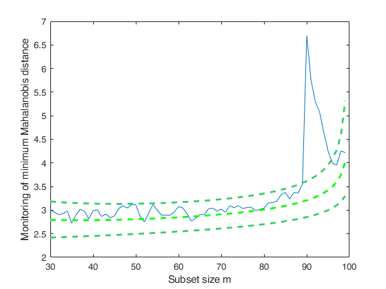
conflev
—confidence interval for the horizontal bands.empty value, vector | struct.
If conflev is empty no confidence line is shown (this is the default).
Confidence interval is based on the chi^2 distribution.
If conflev is a numeric vector it may contain the different confidence level values, e.g.
[0.95,0.99,0.999]. The horizontal confidence lines are shown using red color and line width equal to 2.
If conflev is a structure it is also possible to control the color and the width of the lines associated with the confidence bands. If conflev is a structure it may contain the following fields:
| Value | Description |
|---|---|
color |
Line color, specified as an RGB triplet, (i.e. [0.4 0.6 0.7]) a hexadecimal color code (i.e. #FF8800), a color name (i.e. blue), or a short name (i.e. 'b'). |
linewidth |
scalar, line width of the confidence lines associated with the confidence levels. |
conflev |
numeric vector containing the confidence levels. |
Example: 'conflev',[0.99 0.999]
Data Types: Empty value, vector or struct
Output Arguments
plotopt —options which have been used to create the plot.
Cell array
of strings
Store all options which have been used to generate the plot inside cell plotopt.
References
Atkinson, A.C., Riani, M. and Cerioli, A. (2004), "Exploring multivariate data with the forward search", Springer Verlag, New York.
See Also
|
|
makecontentsfileFS |
malindexplot |
|
|
|
Functions |
|
• The developers of the toolbox • The forward search group • Terms of Use • Acknowledgments