medcouple
MEDCOUPLE computes the medcouple, a robust skewness estimator.
Syntax
Description
Examples
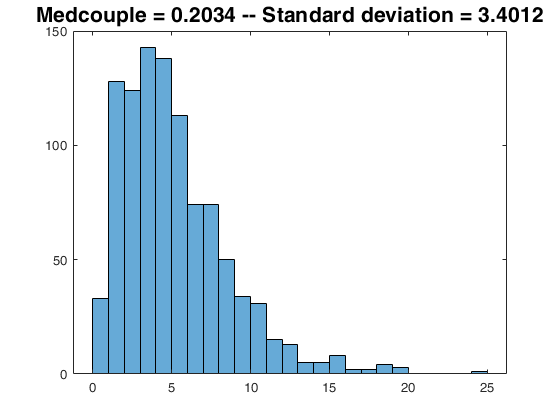
 the fast medcouple (default) on chi2 data.
the fast medcouple (default) on chi2 data.
rng(5);
data = chi2rnd(5,1000,1);
mc1 = medcouple(data);
stddev = std(data);
figure;
histogram(data);
title(['Medcouple = ' num2str(mc1) ' -- Standard deviation = ' num2str(stddev)],'FontSize',16);
The medcouple on small datasets.
The medcouple on small datasets.For small n, it is better to compute the the medcouple also on the reflected sample -z and return (medcouple(z) - medcouple(-z))/2; To work on positive values we do this with:
z = chi2rnd(5,25,1);
mcm = 1; % use naive method (n is small ...)
medoutR = 0.5*(-medcouple(repmat(max(z),size(z,1),1)-z , mcm) + medcouple(z,mcm));
medout  = medcouple(z,mcm);
disp('Application to a non problematic dataset:');
disp(['result with reflected option = ' num2str(medoutR) ' --- result on z only = ' num2str(medoutR)]);
Application to a non problematic dataset:
result with reflected option = -0.1548 --- result on z only = -0.1548
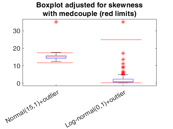
Boxplot using medcouple to adjust for skewness.
Boxplot using medcouple to adjust for skewness.Apply to symmetric and skewed data
rng(5);
%orientation = 'horizontal';
orientation = 'vertical';
% normal data with an outlier
datain1 = 15+randn(200,1);
datain1 = [datain1 ; 35];
% log-normal data with an outlier
datain2 = lognrnd(0,1,200,1);
datain2 = [datain2 ; 35];
k  = 1.5;
% limits on normal data + one outlier
MC_1  = medcouple(datain1);
Q1_1  = quantile(datain1,0.25);
Q3_1  = quantile(datain1,0.75);
IQR_1 = Q3_1 - Q1_1;
DataLimLower_1 = Q1_1 - k * exp(-3.5 * MC_1) * IQR_1;
DataLimUpper_1 = Q3_1 + k * exp(4 * MC_1)    * IQR_1;
% limits on log-normal data + one outlier
MC_2  = medcouple(datain2);
Q1_2  = quantile(datain2,0.25);
Q3_2  = quantile(datain2,0.75);
IQR_2 = Q3_2 - Q1_2;
DataLimLower_2 = Q1_2 - k * exp(-3.5 * MC_2) * IQR_2;
DataLimUpper_2 = Q3_2 + k * exp(4 * MC_2)    * IQR_2;
% boxplot
boxplot([datain1,datain2],'Whisker',k,'Orientation',orientation,...
'OutlierSize',10,'Symbol','*r', ...
'labels',{'Normal(15,1)+outlier','Log-normal(0,1)+outlier'});
title({'Boxplot adjusted for skewness' , 'with medcouple (red limits)'}, 'FontSize' , 20)
set(gca,'FontSize',16);
switch orientation
case 'vertical'
% add the limits (for vertical boxplot)
xx  = xlim(gca);
xx2 = xx/1.1;   xx2(1) = xx(2)/1.5;
xx1 = xx/2; xx1(1) = xx(2)/3.5;
line(xx1,[DataLimLower_1 , DataLimLower_1] , 'Color','red');
line(xx1,[DataLimUpper_1 , DataLimUpper_1] , 'Color','red');
line(xx2,[DataLimLower_2 , DataLimLower_2] , 'Color','red');
line(xx2,[DataLimUpper_2 , DataLimUpper_2] , 'Color','red');
case 'horizontal'
% add the limits (for horizontal boxplot)
yy  = ylim(gca);
yy2 = yy/1.1;   yy2(1) = yy(2)/1.5;
yy1 = yy/2; yy1(1) = yy(2)/3.5;
line([DataLimLower_1 , DataLimLower_1] , yy1,'Color','red');
line([DataLimUpper_1 , DataLimUpper_1] , yy1,'Color','red');
line([DataLimLower_2 , DataLimLower_2] , yy2,'Color','red');
line([DataLimUpper_2 , DataLimUpper_2] , yy2,'Color','red');
end
Related Examples
Assess the perfomance of the various medcouple solutions.
Assess the perfomance of the various medcouple solutions.
% Uses the time execution of the weighted median returned in varargout
% Tm=matlab-fast-quickselectFSw; Tw=matlab-fast-whimed
% Ts=matlab-simplified; To=matlab-octile; Tq=matlab-quantiles;
tm=0; tmmex=0; tw=0; ts=0; to = 0; tq=0;
N      = 800;   % sample size
cycles = 1000;  % number of repetitions
for c = 1:cycles
if mod(c,floor(cycles/10))==0, disp(['repetition n. ' num2str(c)]); end
% Generate different random sequences (seed 896 is a good one to
% compare consistency with the original C code on a difficult sequence)
myseed = randi(1000,1,1);
rng(myseed , 'twister');
datain = rand(N,1);
% REMARK: to generate N random integers (for example between 1 and
% 1000) using the Mersenne Twister in both C and MATLAB, note that the
% line below is equivalent to randi(1000,N,1):
%datain = ceil(datain*1000);
% Line below is to test with skewed data from the lognormal
%datain = lognrnd(0,1,N,1);
% just to ensure that data are stored in a column vector
datain = datain(:);
% $n\log n$, using quickselectFSw
tm0 = tic;
[MCm , t_diva] = medcouple(datain,0,0);
tm  = tm+toc(tm0);
% $n\log n$, using quickselectFSwmex
tm0mex = tic;
[MCmmex , t_diva_mex] = medcouple(datain,0,2);
tmmex  = tmmex+toc(tm0mex);
% $n\log n$, using Haase's weighted median (which is based on MATLAB sortrows)
tw0 = tic;
[MCw , t_Haase] = medcouple(datain,0,1);
tw  = tw+toc(tw0);
% $n^2$ "naive" algorithm, simplified
ts0 = tic;
MCs = medcouple(datain,1);
ts  = ts+toc(ts0);
% Quantiles-based approximation
to0 = tic;
MCo = medcouple(datain,2);
to  = to+toc(to0);
% Octiles-based approximation
tq0 = tic;
MCq = medcouple(datain,3);
tq  = tq+toc(tq0);
end
disp(' ');
disp(['OVERALL TIME EXECUTION IN ' num2str(cycles) ' MC COMPUTATION']);
disp(['time using WM by Haase       = ' num2str(tw)]);
disp(['time using quickselectFSw    = ' num2str(tm)]);
disp(['time using quickselectFSwmex = ' num2str(tmmex)]);
disp(['time using the naive         = ' num2str(ts)]);
disp(['time using quantiles         = ' num2str(tq)]);
disp(['time using octiles           = ' num2str(to)]);
disp(' ');
disp('TIME SPENT IN COMPUTING WEIGHTED AVERAGES IN A SINGLE MC COMPUTATION')
disp(['t_Haase             = ' num2str(t_Haase)]);
disp(['t_quickselectFSw    = ' num2str(t_diva)]);
disp(['t_quickselectFSwmex = ' num2str(t_diva_mex)]);
repetition n. 100
repetition n. 200
repetition n. 300
repetition n. 400
repetition n. 500
repetition n. 600
repetition n. 700
repetition n. 800
repetition n. 900
repetition n. 1000

OVERALL TIME EXECUTION IN 1000 MC COMPUTATION
time using WM by Haase       = 0.88261
time using quickselectFSw    = 0.53556
time using quickselectFSwmex = 0.34337
time using the naive         = 1.6311
time using quantiles         = 0.03368
time using octiles           = 0.073907

TIME SPENT IN COMPUTING WEIGHTED AVERAGES IN A SINGLE MC COMPUTATION
t_Haase             = 0.0005846
t_quickselectFSw    = 0.000214
t_quickselectFSwmex = 7.64e-05
Input Arguments
Output Arguments
More About
References
Brys G., Hubert M. and Struyf A. (2004), A Robust Measure of Skewness, "Journal of Computational and Graphical Statistics", Vol. 13(4), pp. 996-1017.
Hubert M. and Vandervierenb E. (2008), An adjusted boxplot for skewed distributions, "Computational Statistics and Data Analysis", Vol. 52, pp. 5186-5201.
Johnson D.B. and Mizoguchi T. (1978), Selecting the Kth Element in X + Y and X1 + X2 + ... + Xm, "SIAM Journal of Computing", Vol. 7, pp. 147-153.
Hinkley D.V. (1975), On Power Transformations to Symmetry, "Biometrika", Vol. 62, pp.101-111.