tkmeans
tkmeans computes trimmed k-means
Syntax
Description
tkmeans(Y, k, alpha) partitions the points in the n-by-v data matrix Y into k clusters. This partition minimizes the trimmed sum, over all clusters, of the within-cluster sums of point-to-cluster-centroid distances. Rows of Y correspond to points, columns correspond to variables. tkmeans returns inside structure out an n-by-1 vector IDX containing the cluster indices of each point. By default, tkmeans uses (squared) Euclidean distances.
Examples
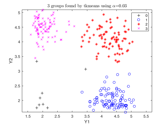
 Trimmed k-means using geyser data (1).
Trimmed k-means using geyser data (1).3 groups and trimming level of 3 percent
close all
Y=load('geyser2.txt');
out=tkmeans(Y,3,0.03,'plots',1);
Total estimated time to complete trimmed k means: 0.35 seconds
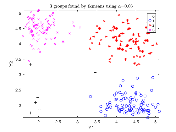
Trimmed k-means using geyser data (2).
option weights =1
close all
Y=load('geyser2.txt');
out=tkmeans(Y,3,0.03,'plots',1,'weights',1);
Trimmed k-means using M5data and different plots.
Weights =1
Y=load('M5data.txt');
close all
out=tkmeans(Y(:,1:2),3,0,'plots',1);
out=tkmeans(Y(:,1:2),3,0.1,'plots','ellipse');
out=tkmeans(Y(:,1:2),3,0.1,'plots','contour');
out=tkmeans(Y(:,1:2),3,0.1,'plots','contourf');
out=tkmeans(Y(:,1:2),3,0.1,'plots','boxplotb');
cascade;
% using a structure for plots
contOpt = struct;
contOpt.cmap = summer
out=tkmeans(Y(:,1:2),3,0.1,'plots',contOpt)
cascade
Related Examples
Trimmed k-means using structured noise.
The data have been generated using the following R instructions set.seed (0) v <- runif (100, -2 * pi, 2 * pi) noise <- cbind (100 + 25 * sin (v), 10 + 5 * v) x <- rbind ( rmvnorm (360, c (0.0, 0), matrix (c (1, 0, 0, 1), ncol = 2)), rmvnorm (540, c (5.0, 10), matrix (c (6, -2, -2, 6), ncol = 2)), noise)
close all
Y=load('structurednoise.txt');
out=tkmeans(Y(:,1:2),2,0.1,'plots',1);
out=tkmeans(Y(:,1:2),5,0.15,'plots',1);
cascade
Trimmed k-means using mixture100 data.
The data have been generated using the following R instructions set.seed (100) mixt <- rbind (rmvnorm (360, c ( 0, 0), matrix (c (1, 0, 0, 1), ncol = 2)), rmvnorm (540, c ( 5, 10), matrix (c (6, -2, -2, 6), ncol = 2)), rmvnorm (100, c (2.5, 5), matrix (c (50, 0, 0, 50), ncol = 2)))
close all
Y=load('mixture100.txt');
out=tkmeans(Y(:,1:2),3,0,'plots',1);
out=tkmeans(Y(:,1:2),2,0.05,'plots',1);
cascade
Input Arguments
Y — Input data.
Matrix.
Data matrix containining n observations on v variables.
Rows of Y represent observations, and columns represent variables.
Missing values (NaN's) and infinite values (Inf's) are allowed, since observations (rows) with missing or infinite values will automatically be excluded from the computations.
Data Types: single| double
alpha — Global trimming level.
Scalar.
alpha is a scalar between 0 and 0.5.
Il alpha = 0 tkmeans reduces to kmeans.
Data Types: single| double
Name-Value Pair Arguments
Specify optional comma-separated pairs of Name,Value arguments.
Name is the argument name and Value
is the corresponding value. Name must appear
inside single quotes (' ').
You can specify several name and value pair arguments in any order as
Name1,Value1,...,NameN,ValueN.
 'nsamp',0
, 'refsteps',20
, 'reftol',0.0001
, 'weights',1
, 'plots', 1
, 'msg',1
, 'nocheck',1
, 'nomes',1
, 'Ysave',1
nsamp
—Number of subsamples.integer.
Number of subsamples which will be extracted to find the partition. If nsamp=0 all subsets will be extracted. They will be (n choose k).
Remark: if the number of all possible subset is <300 the default is to extract all subsets, otherwise just 300.
Example: 'nsamp',0
Data Types: double
refsteps
—Number of iterations.scalar.
Number of refining iterations in each subsample (default = 15).
Example: 'refsteps',20
Data Types: double
reftol
—Tolerance.scalar.
Default value of tolerance for the refining steps. The default value is 1e-14.
Example: 'reftol',0.0001
Data Types: double
weights
—Cluster weights.integer.
A dummy scalar, specifying whether cluster weights (1) shall be considered in the concentration and assignment steps. If weights=1 in the assignment step to the squared Euclidean distance of unit i to group j log n_j is substracted. The default is no cluster weights.
Example: 'weights',1
Data Types: double
plots
—Plot on the screen.scalar, char | struct.
- If plots=0 (default), plots are not generated.
- If plot=1, a plot with the classification is shown on the screen (using the spmplot function). The plot can be: * for v=1, an histogram of the univariate data.
* for v=2, a bivariate scatterplot.
* for v>2, a scatterplot matrix generated by spmplot.
When v>=2 plots offers the following additional features (for v=1 the behaviour is forced to be as for plots=1): - plots='contourf' adds in the background of the bivariate scatterplots a filled contour plot. The colormap of the filled contour is based on grey levels as default.
This argument may also be inserted in a field named 'type' of a structure. In the latter case it is possible to specify the additional field 'cmap', which changes the default colors of the color map used. The field 'cmap' may be a three-column matrix of values in the range [0,1] where each row is an RGB triplet that defines one color.
Check the colormap function for additional informations.
- plots='contour' adds in the background of the bivariate scatterplots a contour plot. The colormap of the contour is based on grey levels as default. This argument may also be inserted in a field named 'type' of a structure.
In the latter case it is possible to specify the additional field 'cmap', which changes the default colors of the color map used. The field 'cmap' may be a three-column matrix of values in the range [0,1] where each row is an RGB triplet that defines one color.
Check the colormap function for additional informations.
- plots='ellipse' superimposes confidence ellipses to each group in the bivariate scatterplots. The size of the ellipse is chi2inv(0.95,2), i.e. the confidence level used by default is 95%. This argument may also be inserted in a field named 'type' of a structure. In the latter case it is possible to specify the additional field 'conflev', which specifies the confidence level to use and it is a value between 0 and 1.
- plots='boxplotb' superimposes on the bivariate scatterplots the bivariate boxplots for each group, using the boxplotb function. This argument may also be inserted in a field named 'type' of a structure.
If plots is a struct it may contain the following fields:
| Value | Description |
|---|---|
type |
a char specifying the type of superimposition Choices are 'contourf', 'contour', 'ellipse' or 'boxplotb'. REMARK - The labels=0 are automatically excluded from the overlaying phase, considering them as outliers. |
Example: 'plots', 1
Data Types: single | double | string
msg
—Message on the screen.scalar.
Scalar which controls whether to display or not messages on the screen. If msg=1 (default) messages are displayed on the screen about estimated time to compute the estimator else no message is displayed on the screen.
Example: 'msg',1
Data Types: double
nocheck
—Check input.scalar.
If nocheck is equal to 1 no check is performed on matrix Y.
As default nocheck=0.
Example: 'nocheck',1
Data Types: double
nomes
—Estimated time message.scalar.
If nomes is equal to 1 no message about estimated time to compute tkemans is displayed, else if nomes is equal to 0 (default), a message about estimated time is displayed.
Example: 'nomes',1
Data Types: double
Ysave
—Saving Y.scalar.
Scalar that is set to 1 to request that the input matrix Y is saved into the output structure out.
Default is 0, i.e. no saving is done.
Example: 'Ysave',1
Data Types: double
Output Arguments
out — description
Structure
Structure which contains the following fields
| Value | Description |
|---|---|
idx |
n-by-1 vector containing assignment of each unit to each of the k groups. Cluster names are integer numbers from 1 to k, 0 indicates trimmed observations. |
muopt |
k-by-v matrix containing cluster centroids locations. Robust estimate of final centroids of the groups. |
sigmaopt |
v-by-v-by-k empirical covariance matrices of the groups found by tkmeans. |
BoxTest |
Structure containing the results of the Box test of equality of covariance matrices. |
bs |
k-by-1 vector containing the units forming initial subset associated with muopt. |
D |
n-by-k matrix containing squared Euclidean distances from each point to every centroid. |
siz |
Matrix of size k-by-3 1st col = sequence from 0 to k 2nd col = number of observations in each cluster 3rd col = percentage of observations in each cluster Remark: 0 denotes unassigned units. |
weights |
Numerical vector of length k, containing the weights of each cluster. If input option weights=1 out.weights=(1/k, ...., 1/k) else if input option weights <> 1 out.weights=(n1/n, ..., nk/n). |
h |
Scalar. Number of observations that have determined the centroids (number of untrimmed units). |
obj |
Scalar. Value of the objective function which is minimized (value of the best returned solution). |
Y |
Original data matrix Y. The field is present only if option Ysave is set to 1. |
emp |
"Empirical" statistics computed on final classification. Scalar or structure. When convergence is reached, out.emp=0. When convergence is not obtained, this field is a structure which contains the statistics of interest: idxemp (ordered from 0 to k*, k* being the number of groups with at least one observation and 0 representing the possible group of outliers), muemp, sigmaemp and sizemp, which are the empirical counterparts of idx, muopt, sigmaopt and siz. |
More About
Additional Details
This iterative algorithm initializes k clusters randomly and performs "concentration steps" in order to improve the current cluster assignment.
The number of maximum concentration steps to be performed is given by input parameter refsteps. For approximately obtaining the global optimum, the system is initialized nsamp times and concentration steps are performed until convergence or refsteps is reached. When processing more complex data sets higher values of nsamp and refsteps have to be specified (obviously implying extra computation time). However, if more then half of the iterations do not converge, a warning message is issued, indicating that nsamp has to be increased.
References
Garcia-Escudero, L.A., Gordaliza, A., Matran, C. and Mayo-Iscar, A. (2008), A General Trimming Approach to Robust Cluster Analysis. Annals of Statistics, Vol. 36, 1324-1345.