wedgeplot
wedgeplot generates the double wedge plot of a time series
Description
Examples
Related Examples
 Example of double wedge plot in series with level shift with option transpose.
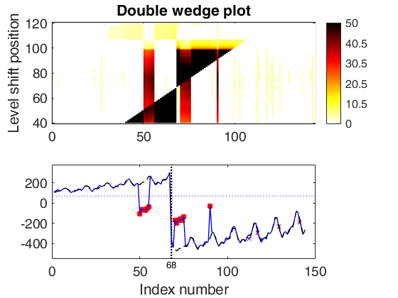
Example of double wedge plot in series with level shift with option transpose.Analysis of contaminated airline data.
% Load the airline data.
%   1949 1950 1951 1952 1953 1954 1955 1956 1957 1958 1959 1960.
y = [112  115  145  171  196  204  242  284  315  340  360  417    % Jan
118  126  150  180  196  188  233  277  301  318  342  391    % Feb
132  141  178  193  236  235  267  317  356  362  406  419    % Mar
129  135  163  181  235  227  269  313  348  348  396  461    % Apr
121  125  172  183  229  234  270  318  355  363  420  472    % May
135  149  178  218  243  264  315  374  422  435  472  535    % Jun
148  170  199  230  264  302  364  413  465  491  548  622    % Jul
148  170  199  242  272  293  347  405  467  505  559  606    % Aug
136  158  184  209  237  259  312  355  404  404  463  508    % Sep
119  133  162  191  211  229  274  306  347  359  407  461    % Oct
104  114  146  172  180  203  237  271  305  310  362  390    % Nov
118  140  166  194  201  229  278  306  336  337  405  432 ]; % Dec
y=(y(:));
% Add a level shift contamintion plus some outliers.
y(50:55)=y(50:55)-300;
y(68:end)=y(68:end)-700;
y(70:75)=y(70:75)+300;
y(90:90)=y(90:90)+300;
% Create structure specifying model
model=struct;
model.trend=2;              % quadratic trend
model.s=12;                 % monthly time series
model.seasonal=204;         % number of harmonics
model.lshift=40:120;        % position where to start monitoring level shift
model.X='';
% Create structure lts specifying lts options
lts=struct;
lts.bestr=20; % number of best solutions to bring to full convergence
% h = dimension of the h subset (75 per cent of the data, bdp=0.25)
[out, varargout]=LTSts(y,'model',model,'nsamp',500,...
'lts',lts,'plots',0,'msg',1);
% Create the double wedge plot.
% Remember to remove the last column of the matrix of the residuals
% obtained for each level shift position if you want to avoid the
% top orange band (just execute RES(:,64)=[] before line 258).
wedgeplot(out,'transpose',true,'extradata',[y out.yhat]);
Level shift for t=40
Level shift for t=41
Level shift for t=42
Level shift for t=43
Level shift for t=44
Level shift for t=45
Level shift for t=46
Level shift for t=47
Level shift for t=48
Level shift for t=49
Level shift for t=50
Level shift for t=51
Level shift for t=52
Level shift for t=53
Level shift for t=54
Level shift for t=55
Level shift for t=56
Level shift for t=57
Level shift for t=58
Level shift for t=59
Level shift for t=60
Level shift for t=61
Level shift for t=62
Level shift for t=63
Level shift for t=64
Level shift for t=65
Level shift for t=66
Level shift for t=67
Level shift for t=68
Level shift for t=69
Level shift for t=70
Level shift for t=71
Level shift for t=72
Level shift for t=73
Level shift for t=74
Level shift for t=75
Level shift for t=76
Level shift for t=77
Level shift for t=78
Level shift for t=79
Level shift for t=80
Level shift for t=81
Level shift for t=82
Level shift for t=83
Level shift for t=84
Level shift for t=85
Level shift for t=86
Level shift for t=87
Level shift for t=88
Level shift for t=89
Level shift for t=90
Level shift for t=91
Level shift for t=92
Level shift for t=93
Level shift for t=94
Level shift for t=95
Level shift for t=96
Level shift for t=97
Level shift for t=98
Level shift for t=99
Level shift for t=100
Level shift for t=101
Level shift for t=102
Level shift for t=103
Level shift for t=104
Level shift for t=105
Level shift for t=106
Level shift for t=107
Level shift for t=108
Level shift for t=109
Level shift for t=110
Level shift for t=111
Level shift for t=112
Level shift for t=113
Level shift for t=114
Level shift for t=115
Level shift for t=116
Level shift for t=117
Level shift for t=118
Level shift for t=119
Level shift for t=120
Input Arguments
Output Arguments
References
Rousseeuw, P.J., Perrotta D., Riani M. and Hubert, M. (2018), Robust Monitoring of Many Time Series with Application to Fraud Detection, "Econometrics and Statistics". [RPRH]