simdatasetreg
simdatasetReg simulates a regression dataset given the parameters of a mixture regression model
Syntax
Description
[y,X,id]=simdatasetreg(n, Pi, Beta, S) generates a regression dataset of size n from a mixture model with parameters 'Pi' (mixing proportions), 'Beta' (matrix of regression coefficients), and 'S' (vector of variances of the distributions of the points around each regression hyperplane). Component sample sizes are produced as a realization from a multinomial distribution with probabilities given by mixing proportions. For example, if n=200, k=4 and Pi=(0.25, 0.25, 0.25, 0.25) function Nk1=mnrnd( n-k, Pi) is used to generate k integer numbers (whose sum is n-k) from the multinomial distribution with parameters n-k and Pi. The size of the groups is given by Nk1+1. The first Nk1(1)+1 observations are generated using vector of regression coefficients Beta(:,1) and variance S(1), ..., and the X simulated as specified in structure Xdistrib, the last Nk1(k)+1 observations are generated using using vector of regression coefficients Beta(:,k), variance S(k) and the X simulated as specified in structure Xdistrib
Generate 2 groups in 4 dimensions and add outliers from uniform distribution.y
=simdatasetreg(n,
Pi,
Beta,
S,
Xdistrib,
Name, Value)
Examples
 Generate mixture of regression.
Generate mixture of regression.Use an average overlapping at centroids = 0.01 and all default options: 1) Beta is generated according to random normal for each group with mu=0 and sigma=1; 2) X in each dimension and each group is generated according to U(0, 1); 3) regression hyperplanes contain intercepts.
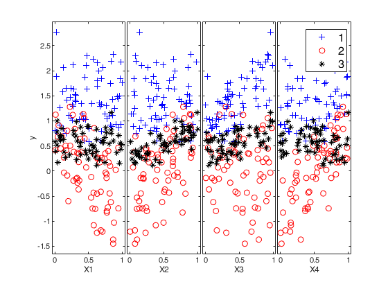
% The value of p includes the intercept
p=5;
k=3;
Q=MixSimreg(k,p,'BarOmega',0.01);
n=200;
% Q.Xdistrib.BarX in this case has dimension 5-by-3 and is equal to
% 1.0000    1.0000    1.0000
% 0.5000    0.5000    0.5000
% 0.5000    0.5000    0.5000
% 0.5000    0.5000    0.5000
% 0.5000    0.5000    0.5000
% Probabilities of overlapping are evaluated at
% Q.Beta(:,1)'*Q.Xdistrib.BarX(:,1) ... Q.Beta(:,3)'*Q.Xdistrib.BarX(:,3)
[y,X,id]=simdatasetreg(n,Q.Pi,Q.Beta,Q.S,Q.Xdistrib);
% spmplot([y X(:,2:end)],id)
yXplot(y,X,'group',id);
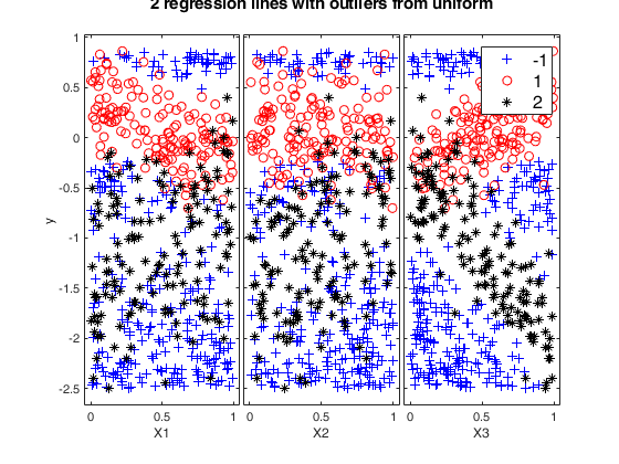
Generate 2 groups in 4 dimensions and add outliers from uniform distribution.
Generate 2 groups in 4 dimensions and add outliers from uniform distribution.
rng('default')
rng(100)
p=4; % p includes the intercept
k=2;
out=MixSimreg(k,p,'BarOmega',0.01);
n=300;
noisevars=0;
noiseunits=300;
[y,X,id]=simdatasetreg(n, out.Pi, out.Beta, out.S, out.Xdistrib,'noisevars',noisevars,'noiseunits',noiseunits);
yXplot(y,X,'group',id);
suplabel('2 regression lines with outliers from uniform','t')
ans =

  Axes (suplabel) with properties:

             XLim: [0 1]
             YLim: [0 1]
           XScale: 'linear'
           YScale: 'linear'
    GridLineStyle: '-'
         Position: [0.0952 0.0863 0.8498 0.8787]
            Units: 'normalized'

  Use GET to show all properties
Generate 4 groups in 4 dimensions and add outliers from uniform distribution.
Generate 4 groups in 4 dimensions and add outliers from uniform distribution.
clear all
close all
rng('default')
rng(10000)
p=2;  % p includes the intercept
k=4;
out=MixSimreg(k,p,'BarOmega',0.01);
n=300;
noisevars=0;
noiseunits=3000;
[y,X,id]=simdatasetreg(n, out.Pi, out.Beta, out.S, out.Xdistrib,'noisevars',noisevars,'noiseunits',noiseunits);
yXplot(y,X,'group',id);
suplabel('2 regression lines with outliers from uniform','t')
ans =

  Axes (suplabel) with properties:

             XLim: [0 1]
             YLim: [0 1]
           XScale: 'linear'
           YScale: 'linear'
    GridLineStyle: '-'
         Position: [0.1055 0.0863 0.8395 0.8787]
            Units: 'normalized'

  Use GET to show all properties
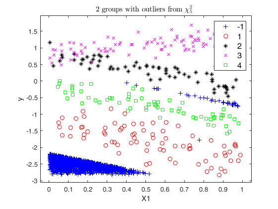
Add outliers generated from Chi2 with 5 degrees of freedom.
Add outliers generated from Chi2 with 5 degrees of freedom.
n=300;
k=4;
p=2;  % p includes the intercept
out=MixSimreg(k,p,'BarOmega',0.01);
noisevars=0;
noiseunits=struct;
noiseunits.number=3000;
% Add asymmetric very concentrated noise
noiseunits.typeout={'Chisquare5'};
[y,X,id]=simdatasetreg(n, out.Pi, out.Beta, out.S, out.Xdistrib,'noisevars',noisevars,'noiseunits',noiseunits);
[H,AX,BigAx]=yXplot(y,X,'group',id);
title(BigAx,'2 groups with outliers from $\chi^2_5$','Interpreter','Latex')
Warning: it was not possible to generate 3000 outliers in 30000 replicates in the interval [1--1] Number of values which was possible to generate is equal to 2848 Please modify the type of outliers using option 'typeout' or increase input option 'alpha' The value of alpha now is 0.001 Outliers have been generated according to Chisquare5 Warning: Output matrix X will have just 3148 rows and not 3300
Related Examples
Add outliers generated from Chi2 with 40 degrees of freedom.
Add outliers generated from Chi2 with 40 degrees of freedom.
n=300;
k=4;
p=2;  % p includes the intercept
out=MixSimreg(k,p,'BarOmega',0.01);
noisevars=0;
noiseunits=struct;
noiseunits.number=3000;
% Add asymmetric concentrated noise
noiseunits.typeout={'Chisquare40'};
[y, X,id]=simdatasetreg(n, out.Pi, out.Beta, out.S, out.Xdistrib,'noisevars',noisevars,'noiseunits',noiseunits);
[H,AX,BigAx]=yXplot(y,X,'group',id);
title(BigAx,'4 groups with outliers from $\chi^2_{40}$','Interpreter','Latex')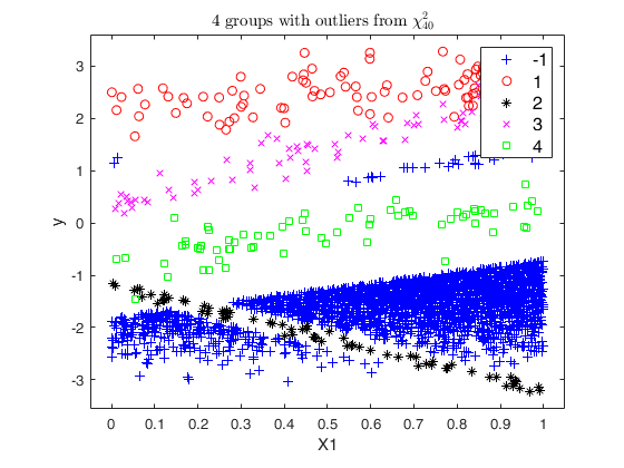
Add outliers generated from normal distribution.
Add outliers generated from normal distribution.
n=300;
k=4;
p=2;  % p includes the intercept
out=MixSimreg(k,p,'BarOmega',0.01);
noisevars=0;
noiseunits=struct;
noiseunits.number=3000;
% Add normal noise
noiseunits.typeout={'normal'};
[y,X,id]=simdatasetreg(n, out.Pi, out.Beta, out.S,out.Xdistrib, 'noisevars',noisevars,'noiseunits',noiseunits);
[H,AX,BigAx]=yXplot(y,X,'group',id);
title(BigAx,'4 groups with outliers from normal distribution','Interpreter','Latex')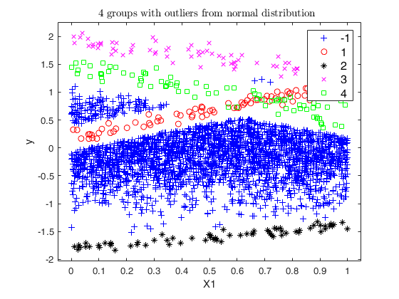
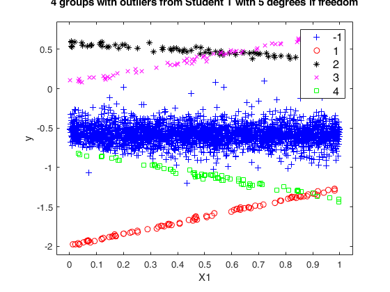
Add outliers generated from Student T with 5 degrees of freedom.
Add outliers generated from Student T with 5 degrees of freedom.
n=300;
k=4;
p=2;  % p includes the intercept
out=MixSimreg(k,p,'BarOmega',0.01);
noisevars=0;
noiseunits=struct;
noiseunits.number=3000;
% Add outliers from T5
noiseunits.typeout={'T5'};
[y, X,id]=simdatasetreg(n, out.Pi, out.Beta, out.S,out.Xdistrib, 'noisevars',noisevars,'noiseunits',noiseunits);
[H,AX,BigAx]=yXplot(y,X,'group',id);
suplabel('4 groups with outliers from Student T with 5 degrees if freedom','t')
ans =

  Axes (suplabel) with properties:

             XLim: [0 1]
             YLim: [0 1]
           XScale: 'linear'
           YScale: 'linear'
    GridLineStyle: '-'
         Position: [0.1055 0.0863 0.8395 0.8787]
            Units: 'normalized'

  Use GET to show all properties
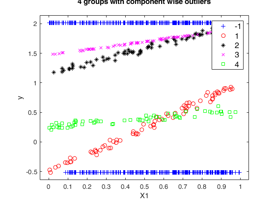
Add componentwise contamination.
Add componentwise contamination.
n=300;
k=4;
p=2;  % p includes the intercept
out=MixSimreg(k,p,'BarOmega',0.01);
noisevars='';
noiseunits=struct;
noiseunits.number=3000;
% Add asymmetric concentrated noise
noiseunits.typeout={'componentwise'};
[y, X,id]=simdatasetreg(n, out.Pi, out.Beta, out.S,out.Xdistrib, 'noisevars',noisevars,'noiseunits',noiseunits);
yXplot(y,X,'group',id);
suplabel('4 groups with component wise outliers','t')
ans =

  Axes (suplabel) with properties:

             XLim: [0 1]
             YLim: [0 1]
           XScale: 'linear'
           YScale: 'linear'
    GridLineStyle: '-'
         Position: [0.1055 0.0863 0.8395 0.8787]
            Units: 'normalized'

  Use GET to show all properties
Add outliers generated from Chisquare and T distribution.
Add outliers generated from Chisquare and T distribution.
n=300;
k=4;
p=2;  % p includes the intercept
out=MixSimreg(k,p,'BarOmega',0.01);
noisevars=0;
noiseunits=struct;
noiseunits.number=5000*ones(2,1);
noiseunits.typeout={'Chisquare3','T20'};
[y, X,id]=simdatasetreg(n, out.Pi, out.Beta, out.S, out.Xdistrib, 'noisevars',noisevars,'noiseunits',noiseunits);
[H,AX,BigAx]=yXplot(y,X,'group',id);
title(BigAx,'4 groups with outliers from $\chi^2_{3}$ and $T_{20}$','Interpreter','Latex')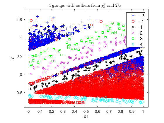
Add outliers from Chisquare and T distribution and use a personalized value of alpha.
Add outliers from Chisquare and T distribution and use a personalized value of alpha.
n=300;
k=4;
p=2;  % p includes the intercept
out=MixSimreg(k,p,'BarOmega',0.01);
noisevars=0;
noiseunits=struct;
noiseunits.number=5000*ones(2,1);
noiseunits.typeout={'Chisquare3','T20'};
noiseunits.alpha=0.002;
[y, X,id]=simdatasetreg(n, out.Pi, out.Beta, out.S, out.Xdistrib, 'noisevars',noisevars,'noiseunits',noiseunits);
[H,AX,BigAx]=yXplot(y,X,'group',id);
title(BigAx,'4 groups with outliers from $\chi^2_{3}$ and $T_{20}$','Interpreter','Latex')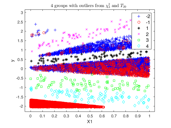
Add outliers from Chi2 and point mass contamination and add one noise variable.
Add outliers from Chi2 and point mass contamination and add one noise variable.
n=300;
k=4;
p=2;  % p includes the intercept
out=MixSimreg(k,p,'BarOmega',0.01);
noisevars=struct;
noisevars.number=1;
noiseunits=struct;
noiseunits.number=[100 100];
noiseunits.typeout={'pointmass' 'Chisquare5'};
[y, X,id]=simdatasetreg(n, out.Pi, out.Beta, out.S, out.Xdistrib, 'noisevars',noisevars,'noiseunits',noiseunits);
[H,AX,BigAx]=yXplot(y,X,'group',id);
title(BigAx,'4 groups with outliers from $\chi^2_{5}$ and point mass $+1$ noise var','Interpreter','Latex')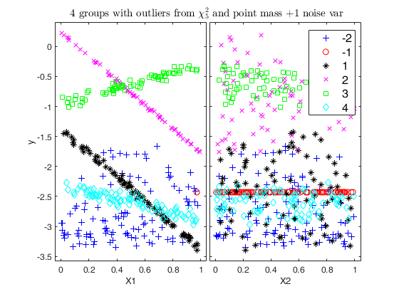
Example of the use of personalized interval to generate outliers.
Example of the use of personalized interval to generate outliers.
n=300;
k=4;
p=2;  % p includes the intercept
out=MixSimreg(k,p,'BarOmega',0.01);
noiseunits=struct;
noiseunits.number=1000;
noiseunits.typeout={'uniform'};
% Generate outliers in the interval [-1 1] for the first variable and
% interval [1 2] for the second variable
noiseunits.interval=[-1 1;
1 2];
% Finally add a noise variable
noisevars=struct;
noisevars.number=1;
[y, X,id]=simdatasetreg(n, out.Pi, out.Beta, out.S, out.Xdistrib, 'noisevars',noisevars,'noiseunits',noiseunits);
[H,AX,BigAx]=yXplot(y,X,'group',id);
title(BigAx,'4 groups with outliers from uniform using a personalized interval $+1$ noise var','Interpreter','Latex')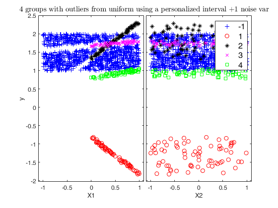
Example with user defined explanatory variables values (1).
Example with user defined explanatory variables values (1).Here the X distribution is the same for each component.
clear all
close all
rng(1234,'twister');
% mixture parameters
intercept = 0; % 1/0 = intercept yes/no
p=1+intercept;
k=2;
n=200;
% beta distributed as halfnormal
betadistrib=struct;
betadistrib.type='HalfNormal';
betadistrib.sigma=3;
% explanatory variables distribution chosen by the User from a beta
XdistribB=struct;
XdistribB.intercept=intercept;
XdistribB.type='User';
X1=random('beta',1,5,n,1);             % data generation: user distribution is a beta
XdistribB.BarX = ones(1,k)*mean(X1);   % mean of the generated data: one per group
% overlap level baromega: chosen at random here, in a given range
mino = 0.01; maxo = 0.1;
baromega = mino + (maxo-mino).*rand(1,1);
% estimated mixsim parameters
Q=MixSimreg(k,p,'BarOmega',baromega,'Xdistrib',XdistribB,'betadistrib',betadistrib);
% Simulate the data from the mixim parameters and the user values for X
if intercept
Q.Xdistrib.X = [ones(n,1) X1];
else
Q.Xdistrib.X = X1;
end
[y,X,id]=simdatasetreg(n,Q.Pi,Q.Beta,Q.S,Q.Xdistrib);
yXplot(y,X,'group',id,'tag','X_beta');
set(gcf,'Name','X Beta distributed');
title('User-defined distribution for X');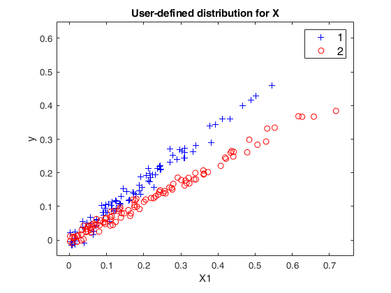
Example with user defined explanatory variables values (2).
Example with user defined explanatory variables values (2).Here the X distribution is specific for each component.
clear all
close all
rng(12345,'twister');
% mixture parameters
intercept = 0;      % 1/0 = intercept yes/no
n=200;
p=1+intercept;
k=2;                %do not change k: it would not work (see below to generalise)
% beta distributed as halfnormal
betadistrib=struct;
betadistrib.type='HalfNormal';
betadistrib.sigma=3;
% explanatory variables distribution chosen by the User from a beta
XdistribB=struct;
XdistribB.intercept=intercept;
XdistribB.type='User';
%for i=1:10
% X beta distributed
X2=random('beta',0.5,1,n,1);
muBeta2 = mean(X2);
X1=random('beta',1,0.5,n,1);
muBeta1 = mean(X1);
% data generation: user distribution is a beta
XdistribB.BarX = [muBeta1 muBeta2]; % mean of the generated data: one per group
% overlap level baromega: chosen at random here, in a given range
mino = 0.01; maxo = 0.05;
maxomega = mino + (maxo-mino).*rand(1,1);
% estimated mixsim parameters
Q=MixSimreg(k,p,'hom',true,'MaxOmega',maxomega,'Xdistrib',XdistribB,'betadistrib',betadistrib);
% Simulate the data from the mixim parameters and the user values for X
if intercept
Q.Xdistrib.X = [ones(k*n,1) , [X1 ; X2]];
else
Q.Xdistrib.X = [X1 ; X2];
end
[y,X,id]=simdatasetreg(k*n,Q.Pi,Q.Beta,Q.S,Q.Xdistrib);
yXplot(y,X,'group',id,'tag','X_beta');
set(gcf,'Name','X Beta distributed');
title('User-defined distribution for X');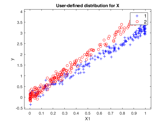
Input Arguments
Output Arguments
More About
References
Maitra, R. and Melnykov, V. (2010), Simulating data to study performance of finite mixture modeling and clustering algorithms, "The Journal of Computational and Graphical Statistics", Vol. 19, pp. 354-376. [to refer to this publication we will use "MM2010 JCGS"]
Melnykov, V., Chen, W.-C. and Maitra, R. (2012), MixSim: An R Package for Simulating Data to Study Performance of Clustering Algorithms, "Journal of Statistical Software", Vol. 51, pp. 1-25.
Davies, R. (1980), The distribution of a linear combination of chi-square random variables, "Applied Statistics", Vol. 29, pp. 323-333.