CorAnaplot

CorAnaplot draws customized Correspondence Analysis (CA) graphs

expand all in page

Syntax

CorAnaplot(out)example
CorAnaplot(out,Name,Value)example

Description

example

CorAnaplot(out) CorAnaplot with all the default options.

example

CorAnaplot(out, Name, Value) CorAnaplot with personalized symbols.

Examples

expand all

CorAnaplot with all the default options.

Prepare the data.

N=[51	64	32	29	17	59	66	70;
53	90	78	75	22	115	117	86;
71	111	50	40	11	79	88	177;
1	7	5	5	4	9	8	5;
7	11	4	3	2	2	17	18;
7	13	12	11	11	18	19	17;
21	37	14	26	9	14	34	61;
12	35	19	6	7	21	30	28;
10	7	7	3	1	8	12	8;
4	7	7	6	2	7	6	13;
8	22	7	10	5	10	27	17;
25	45	38	38	13	48	59	52;
18	27	20	19	9	13	29	53;
35	61	29	14	12	30	63	58;
2	4	3	1	4	nan  nan	nan	  ;
2	8	2	5	2	nan  nan	nan;
1	5	4	6	3	nan  nan	nan;
3	3	1	3	4	nan  nan	nan];
% rowslab = cell containing row labels
rowslab={'money','future','unemployment','circumstances',...
'hard','economic','egoism','employment','finances',...
'war','housing','fear','health','work','comfort','disagreement',...
'world','to_live'};
% colslab = cell containing column labels
colslab={'unqualified','cep','bepc','high_school_diploma','university',...
'thirty','fifty','more_fifty'};
if verLessThan('matlab','8.2.0')==0
tableN=array2table(N,'VariableNames',colslab,'RowNames',rowslab);
% Extract just active rows
Nactive=tableN(1:14,1:5);
Nsupr=tableN(15:18,1:5);
Nsupc=tableN(1:14,6:8);
Sup=struct;
Sup.r=Nsupr;
Sup.c=Nsupc;
% Compute Correspondence analysis
else
Nactive=N(1:14,1:5);
Lr=rowslab(1:14);
Lc=colslab(1:5);
Sup=struct;
Sup.r=N(15:end,1:5);
Sup.Lr=rowslab(15:end);
Sup.c=N(1:14,6:8);
Sup.Lc=colslab(6:8);
end
% Compute correspondence analysis
out=CorAna(Nactive,'Sup',Sup,'plots',0,'dispresults',false);
% Show the correspondence analysis plot.
% Rows and columns are shown in principal coordinates
CorAnaplot(out)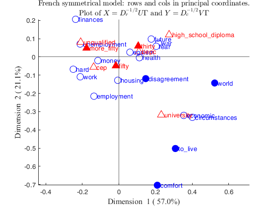

Click here for the graphical output of this example (link to Ro.S.A. website).

CorAnaplot with personalized symbols.

close all
% Prepare the data.
N=[51	64	32	29	17	59	66	70;
53	90	78	75	22	115	117	86;
71	111	50	40	11	79	88	177;
1	7	5	5	4	9	8	5;
7	11	4	3	2	2	17	18;
7	13	12	11	11	18	19	17;
21	37	14	26	9	14	34	61;
12	35	19	6	7	21	30	28;
10	7	7	3	1	8	12	8;
4	7	7	6	2	7	6	13;
8	22	7	10	5	10	27	17;
25	45	38	38	13	48	59	52;
18	27	20	19	9	13	29	53;
35	61	29	14	12	30	63	58;
2	4	3	1	4	nan  nan	nan	  ;
2	8	2	5	2	nan  nan	nan;
1	5	4	6	3	nan  nan	nan;
3	3	1	3	4	nan  nan	nan];
% rowslab = cell containing row labels
rowslab={'money','future','unemployment','circumstances',...
'hard','economic','egoism','employment','finances',...
'war','housing','fear','health','work','comfort','disagreement',...
'world','to_live'};
% colslab = cell containing column labels
colslab={'unqualified','cep','bepc','high_school_diploma','university',...
'thirty','fifty','more_fifty'};
if verLessThan('matlab','8.2.0')==0
tableN=array2table(N,'VariableNames',colslab,'RowNames',rowslab);
% Extract just active rows
Nactive=tableN(1:14,1:5);
Nsupr=tableN(15:18,1:5);
Nsupc=tableN(1:14,6:8);
Sup=struct;
Sup.r=Nsupr;
Sup.c=Nsupc;
% Compute Correspondence analysis
else
Nactive=N(1:14,1:5);
Lr=rowslab(1:14);
Lc=colslab(1:5);
Sup=struct;
Sup.r=N(15:end,1:5);
Sup.Lr=rowslab(15:end);
Sup.c=N(1:14,6:8);
Sup.Lc=colslab(6:8);
end
% Six-pointed star (hesagram) for supplementary rows
SymbolRows='h';
% Five-pointed star (pentagram) for supplementary rows
SymbolRowsSup='p';
% Color for active rows
ColorRows='b';
% Color for supplementary rows (dark blue)
ColorRowsSup=[6 13 123]/255;
% Blue fill color for active rows
MarkerFaceColorRows='b';
% Right-pointing triangle for active columns
Symbolcols='^';
% Six-pointed star (hexagram) for supplementary columns
SymbolcolsSup='h';
% Color for active columns
ColorCols='r';
% Red fill color for active rows
MarkerFaceColorCols='r';
% Color for supplementary columns (dark red)
ColorColsSup=[128 0 0]/255;
plots=struct;
plots.SymbolRows=SymbolRows;
plots.SymbolRowsSup=SymbolRowsSup;
plots.ColorRows=ColorRows;
plots.ColorRowsSup=ColorRowsSup;
plots.MarkerFaceColorRows=MarkerFaceColorRows;
plots.SymbolCols=Symbolcols;
plots.SymbolColsSup=SymbolcolsSup;
plots.ColorCols=ColorCols;
plots.ColorColsSup=ColorColsSup;
plots.MarkerFaceColorCols=MarkerFaceColorCols;
% change the sign of the second dimension
changedimsign=[false true];
out=CorAna(Nactive,'Sup',Sup,'plots',0,'dispresults',false);
CorAnaplot(out,'plots',plots,'changedimsign',changedimsign)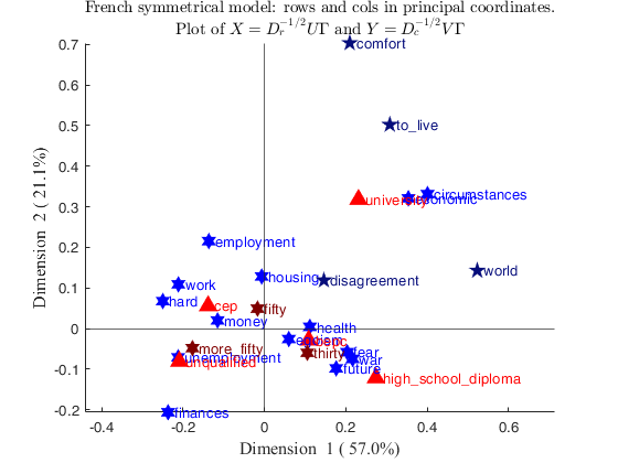

Related Examples

expand all

CorAnaplot with personalized displacement.

close all
% Prepare the data.
N=[51	64	32	29	17	59	66	70;
53	90	78	75	22	115	117	86;
71	111	50	40	11	79	88	177;
1	7	5	5	4	9	8	5;
7	11	4	3	2	2	17	18;
7	13	12	11	11	18	19	17;
21	37	14	26	9	14	34	61;
12	35	19	6	7	21	30	28;
10	7	7	3	1	8	12	8;
4	7	7	6	2	7	6	13;
8	22	7	10	5	10	27	17;
25	45	38	38	13	48	59	52;
18	27	20	19	9	13	29	53;
35	61	29	14	12	30	63	58;
2	4	3	1	4	nan  nan	nan	  ;
2	8	2	5	2	nan  nan	nan;
1	5	4	6	3	nan  nan	nan;
3	3	1	3	4	nan  nan	nan];
% rowslab = cell containing row labels
rowslab={'money','future','unemployment','circumstances',...
'hard','economic','egoism','employment','finances',...
'war','housing','fear','health','work','comfort','disagreement',...
'world','to_live'};
% colslab = cell containing column labels
colslab={'unqualified','cep','bepc','high_school_diploma','university',...
'thirty','fifty','more_fifty'};
if verLessThan('matlab','8.2.0')==0
tableN=array2table(N,'VariableNames',colslab,'RowNames',rowslab);
% Extract just active rows
Nactive=tableN(1:14,1:5);
Nsupr=tableN(15:18,1:5);
Nsupc=tableN(1:14,6:8);
Sup=struct;
Sup.r=Nsupr;
Sup.c=Nsupc;
% Compute Correspondence analysis
else
Nactive=N(1:14,1:5);
Lr=rowslab(1:14);
Lc=colslab(1:5);
Sup=struct;
Sup.r=N(15:end,1:5);
Sup.Lr=rowslab(15:end);
Sup.c=N(1:14,6:8);
Sup.Lc=colslab(6:8);
end
% No horizontal displacement for the labels.
addx=0;
out=CorAna(Nactive,'Sup',Sup,'plots',0,'dispresults',false);
CorAnaplot(out,'addx',addx)

Correspondence analysis plot with selected ellipses.

N=[51	64	32	29	17	59	66	70;
53	90	78	75	22	115	117	86;
71	111	50	40	11	79	88	177;
1	7	5	5	4	9	8	5;
7	11	4	3	2	2	17	18;
7	13	12	11	11	18	19	17;
21	37	14	26	9	14	34	61;
12	35	19	6	7	21	30	28;
10	7	7	3	1	8	12	8;
4	7	7	6	2	7	6	13;
8	22	7	10	5	10	27	17;
25	45	38	38	13	48	59	52;
18	27	20	19	9	13	29	53;
35	61	29	14	12	30	63	58;
2	4	3	1	4	nan  nan	nan	  ;
2	8	2	5	2	nan  nan	nan;
1	5	4	6	3	nan  nan	nan;
3	3	1	3	4	nan  nan	nan];
% rowslab = cell containing row labels
rowslab={'money','future','unemployment','circumstances',...
'hard','economic','egoism','employment','finances',...
'war','housing','fear','health','work','comfort','disagreement',...
'world','to_live'};
% colslab = cell containing column labels
colslab={'unqualified','cep','bepc','high_school_diploma','university',...
'thirty','fifty','more_fifty'};
if verLessThan('matlab','8.2.0')==0
tableN=array2table(N,'VariableNames',colslab,'RowNames',rowslab);
% Extract just active rows
Nactive=tableN(1:14,1:5);
Nsupr=tableN(15:18,1:5);
Nsupc=tableN(1:14,6:8);
Sup=struct;
Sup.r=Nsupr;
Sup.c=Nsupc;
else
Nactive=N(1:14,1:5);
Lr=rowslab(1:14);
Lc=colslab(1:5);
Sup=struct;
Sup.r=N(15:end,1:5);
Sup.Lr=rowslab(15:end);
Sup.c=N(1:14,6:8);
Sup.Lc=colslab(6:8);
end
% Superimpose confidence ellipses for rows 2 and 4 and for column 3
confellipse=struct;
confellipse.selRows=[2 4];
% Ellipse for column 3 using an integer
confellipse.selCols=3;
% Ellipse for column 3 using a Boolean vector
confellipse.selCols=[ false false true false false];
% confellipse.selCols={'c3'};
% Use the 3 methods below in order to compute the confidence ellipses for
% the selected rows and columns of the input contingency table
confellipse.method={'multinomial' 'bootRows' 'bootCols'};
% Set number of simulations
confellipse.nsimul=500;
% Set confidence interval
confellipse.conflev=0.50;
out=CorAna(Nactive,'Sup',Sup,'plots',0,'dispresults',false);
% Draw correspondence analysis plot with requested confidence ellipses
CorAnaplot(out,'plots',1,'confellipse',confellipse)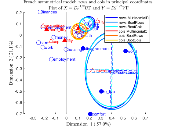

Correspondence analysis plot with ellipses only on column points.

N=[51	64	32	29	17	59	66	70;
53	90	78	75	22	115	117	86;
71	111	50	40	11	79	88	177;
1	7	5	5	4	9	8	5;
7	11	4	3	2	2	17	18;
7	13	12	11	11	18	19	17;
21	37	14	26	9	14	34	61;
12	35	19	6	7	21	30	28;
10	7	7	3	1	8	12	8;
4	7	7	6	2	7	6	13;
8	22	7	10	5	10	27	17;
25	45	38	38	13	48	59	52;
18	27	20	19	9	13	29	53;
35	61	29	14	12	30	63	58;
2	4	3	1	4	nan  nan	nan	  ;
2	8	2	5	2	nan  nan	nan;
1	5	4	6	3	nan  nan	nan;
3	3	1	3	4	nan  nan	nan];
% rowslab = cell containing row labels
rowslab={'money','future','unemployment','circumstances',...
'hard','economic','egoism','employment','finances',...
'war','housing','fear','health','work','comfort','disagreement',...
'world','to_live'};
% colslab = cell containing column labels
colslab={'unqualified','cep','bepc','high_school_diploma','university',...
'thirty','fifty','more_fifty'};
if verLessThan('matlab','8.2.0')==0
tableN=array2table(N,'VariableNames',colslab,'RowNames',rowslab);
% Extract just active rows
Nactive=tableN(1:14,1:5);
Nsupr=tableN(15:18,1:5);
Nsupc=tableN(1:14,6:8);
Sup=struct;
Sup.r=Nsupr;
Sup.c=Nsupc;
else
Nactive=N(1:14,1:5);
Lr=rowslab(1:14);
Lc=colslab(1:5);
Sup=struct;
Sup.r=N(15:end,1:5);
Sup.Lr=rowslab(15:end);
Sup.c=N(1:14,6:8);
Sup.Lc=colslab(6:8);
end
% Superimpose confidence ellipses
confellipse=struct;
% No confidence ellipse for row points
confellipse.selRows=[];
% Ellipse for all the column points using a Boolean vector
confellipse.selCols=[ true true true true true];
% Compare methods 'multinomial' and 'bootCols'
confellipse.method={'multinomial' 'bootCols'};
% Set number of simulations
confellipse.nsimul=10000;
% Set confidence interval
confellipse.conflev=0.90;
out=CorAna(Nactive,'Sup',Sup,'plots',0,'dispresults',false);
% Draw correspondence analysis plot with requested confidence ellipses
CorAnaplot(out,'plots',1,'confellipse',confellipse)

Correspondence analysis plot using latent dimensions 3 and 4.

N=[51	64	32	29	17	59	66	70;
53	90	78	75	22	115	117	86;
71	111	50	40	11	79	88	177;
1	7	5	5	4	9	8	5;
7	11	4	3	2	2	17	18;
7	13	12	11	11	18	19	17;
21	37	14	26	9	14	34	61;
12	35	19	6	7	21	30	28;
10	7	7	3	1	8	12	8;
4	7	7	6	2	7	6	13;
8	22	7	10	5	10	27	17;
25	45	38	38	13	48	59	52;
18	27	20	19	9	13	29	53;
35	61	29	14	12	30	63	58;
2	4	3	1	4	nan  nan	nan	  ;
2	8	2	5	2	nan  nan	nan;
1	5	4	6	3	nan  nan	nan;
3	3	1	3	4	nan  nan	nan];
% rowslab = cell containing row labels
rowslab={'money','future','unemployment','circumstances',...
'hard','economic','egoism','employment','finances',...
'war','housing','fear','health','work','comfort','disagreement',...
'world','to_live'};
% colslab = cell containing column labels
colslab={'unqualified','cep','bepc','high_school_diploma','university',...
'thirty','fifty','more_fifty'};
if verLessThan('matlab','8.2.0')==0
tableN=array2table(N,'VariableNames',colslab,'RowNames',rowslab);
% Extract just active rows
Nactive=tableN(1:14,1:5);
Nsupr=tableN(15:18,1:5);
Nsupc=tableN(1:14,6:8);
Sup=struct;
Sup.r=Nsupr;
Sup.c=Nsupc;
else
Nactive=N(1:14,1:5);
Lr=rowslab(1:14);
Lc=colslab(1:5);
Sup=struct;
Sup.r=N(15:end,1:5);
Sup.Lr=rowslab(15:end);
Sup.c=N(1:14,6:8);
Sup.Lc=colslab(6:8);
end
% Superimpose ellipses
confellipse=struct;
% Ellipse for the first 3 row points
confellipse.selRows=1:3;
% Ellipse for selected column points using a Boolean vector
confellipse.selCols=[ false false true true false];
% Compare methods 'multinomial' and 'bootCols'
confellipse.method={'multinomial' 'bootCols'};
% Set number of simulations
confellipse.nsimul=10000;
% Set confidence interval
confellipse.conflev=0.90;
d1=3;
d2=4;
out=CorAna(Nactive,'Sup',Sup,'plots',0,'dispresults',false,'d1',d1,'d2',d2);
% Draw correspondence analysis plot with requested confidence ellipses
CorAnaplot(out,'plots',1,'confellipse',confellipse,'d1',d1,'d2',d2)

Correspondence analysis of the smoke data.

In this example we compare the results which are obtained using option plots.alpha='colprincipal'; (which implicitly implies alpha=0) with those which come out imposing directly plots.alpha=0.

load smoke
[N,~,~,labels]=crosstab(smoke{:,1},smoke{:,2});
[I,J]=size(N);
labels_rows=labels(1:I,1);
labels_columns=labels(1:J,2);
out=CorAna(N,'Lr',labels_rows,'Lc',labels_columns,'plots',0,'dispresults',false);
plots=struct;
plots.alpha='rowgab';
plots.alpha='colgab';
plots.alpha='rowgreen';
plots.alpha='colgreen';
% Add confidence ellipses
confellipse=1;
plots.alpha='bothprincipal';
plots.alpha='rowprincipal';
plots.alpha='colprincipal';
h1=subplot(1,2,1);
CorAnaplot(out,'plots',plots,'confellipse',confellipse,'h',h1)
h2=subplot(1,2,2);
plots.alpha=0;
CorAnaplot(out,'plots',plots,'confellipse',confellipse,'h',h2);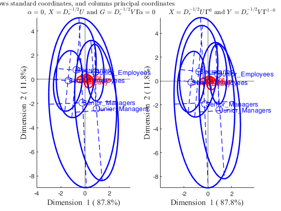

Correspondence analysis of the car dataset.

load car
out=CorAna(car,'plots',0);
plots=struct;
% Color of Row labels proportional to the amount of inertia which is
% explained by the the two latent dimensions (communalities)
plots.ColorMapLabelRows= 'CntrbDim2In';
CorAnaplot(out,'plots',plots)

An example with personalized colormap in option plots.

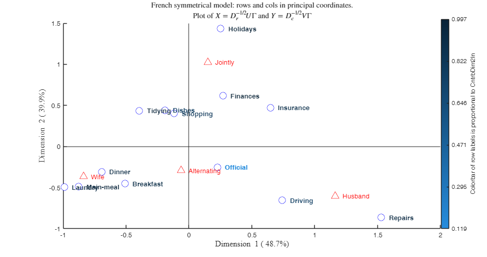
load housetasks.mat
out=CorAna(housetasks,'plots',0);
% Show a colorbar which is proportional to the contribution of the first
% two latent dimensions to the inertia of each
% Use colorbar abyss in a reverse order, that is in such a way that
% the darkest blue colors are associated with points with high communalities
plots=struct;
plots.ColorMapLabelRows= 'CntrbDim2In';
plots.ColorMap=flipud(abyss);
CorAnaplot(out,'plots',plots)
% From the plot it is clear that the RowPoint "Official" has an inertia which
% is not explained by the first two latent dimensions.
disp(out.OverviewRows(:,["CntrbDim2In_1" "CntrbDim2In_2"]))

Summary
             Singular_value    Inertia    Accounted_for    Cumulative
             ______________    _______    _____________    __________

    dim_1       0.73681        0.54289       0.48692        0.48692  
    dim_2       0.66709          0.445       0.39913        0.88605  
    dim_3       0.35644        0.12705       0.11395              1  

ROW POINTS
Results for dimension: 1
                  Scores     CntrbPnt2In    CntrbDim2In
                 ________    ___________    ___________

    Laundry      -0.99184       0.18287       0.73999  
    Main-meal    -0.87559       0.12389        0.7416  
    Dinner       -0.69257      0.054714       0.77664  
    Breakfast     -0.5086      0.038249       0.50494  
    Tidying      -0.39381      0.019984       0.43981  
    Dishes       -0.18896     0.0042617       0.11812  
    Shopping     -0.11768     0.0017552      0.063654  
    Official      0.22663     0.0052078      0.053045  
    Driving       0.74177      0.080778       0.43202  
    Finances      0.27077     0.0087501       0.16068  
    Insurance     0.64708      0.061471       0.57601  
    Repairs        1.5288        0.4073       0.70674  
    Holidays      0.25249      0.010773      0.029792  

Results for dimension: 2
                  Scores     CntrbPnt2In    CntrbDim2In
                 ________    ___________    ___________

    Laundry      -0.49532      0.055639       0.18455  
    Main-meal    -0.49011      0.047355       0.23236  
    Dinner        -0.3081       0.01321        0.1537  
    Breakfast     -0.4528      0.036986       0.40023  
    Tidying       0.43434      0.029656       0.53502  
    Dishes        0.44197      0.028441       0.64615  
    Shopping      0.40332      0.025152       0.74766  
    Official     -0.25361     0.0079562      0.066426  
    Driving      -0.65341      0.076469       0.33523  
    Finances      0.61787      0.055585       0.83667  
    Insurance     0.47378      0.040204        0.3088  
    Repairs      -0.86426       0.15881       0.22587  
    Holidays        1.435       0.42454       0.96236  

COLUMN POINTS
Results for dimension: 1
                    Scores      CntrbPnt2In    CntrbDim2In
                   _________    ___________    ___________

    Wife            -0.83762       0.44462        0.80188 
    Alternating    -0.062185     0.0010374      0.0047799 
    Husband           1.1609       0.54234        0.77203 
    Jointly          0.14943      0.012004       0.020706 

Results for dimension: 2
                    Scores     CntrbPnt2In    CntrbDim2In
                   ________    ___________    ___________

    Wife           -0.36522      0.10312        0.15245  
    Alternating    -0.29159     0.027828         0.1051  
    Husband        -0.60192      0.17787        0.20754  
    Jointly          1.0266      0.69118        0.97729  

-----------------------------------------------------------
Overview ROW POINTS
                   Mass      Score_1     Score_2     Inertia     CntrbPnt2In_1    CntrbPnt2In_2    CntrbDim2In_1    CntrbDim2In_2
                 ________    ________    ________    ________    _____________    _____________    _____________    _____________

    Laundry       0.10092    -0.99184    -0.49532     0.13416        0.18287         0.055639         0.73999          0.18455   
    Main-meal    0.087729    -0.87559    -0.49011    0.090692        0.12389         0.047355          0.7416          0.23236   
    Dinner       0.061927    -0.69257     -0.3081    0.038246       0.054714          0.01321         0.77664           0.1537   
    Breakfast    0.080275     -0.5086     -0.4528    0.041124       0.038249         0.036986         0.50494          0.40023   
    Tidying      0.069954    -0.39381     0.43434    0.024667       0.019984         0.029656         0.43981          0.53502   
    Dishes       0.064794    -0.18896     0.44197    0.019587      0.0042617         0.028441         0.11812          0.64615   
    Shopping     0.068807    -0.11768     0.40332     0.01497      0.0017552         0.025152        0.063654          0.74766   
    Official     0.055046     0.22663    -0.25361      0.0533      0.0052078        0.0079562        0.053045         0.066426   
    Driving      0.079702     0.74177    -0.65341     0.10151       0.080778         0.076469         0.43202          0.33523   
    Finances     0.064794     0.27077     0.61787    0.029564      0.0087501         0.055585         0.16068          0.83667   
    Insurance    0.079702     0.64708     0.47378    0.057936       0.061471         0.040204         0.57601           0.3088   
    Repairs       0.09461      1.5288    -0.86426     0.31287         0.4073          0.15881         0.70674          0.22587   
    Holidays     0.091743     0.25249       1.435     0.19631       0.010773          0.42454        0.029792          0.96236   

Overview COLUMN POINTS
                    Mass       Score_1     Score_2     Inertia    CntrbPnt2In_1    CntrbPnt2In_2    CntrbDim2In_1    CntrbDim2In_2
                   _______    _________    ________    _______    _____________    _____________    _____________    _____________

    Wife           0.34404     -0.83762    -0.36522    0.30102        0.44462         0.10312           0.80188         0.15245   
    Alternating    0.14564    -0.062185    -0.29159    0.11782      0.0010374        0.027828         0.0047799          0.1051   
    Husband        0.21846       1.1609    -0.60192    0.38137        0.54234         0.17787           0.77203         0.20754   
    Jointly        0.29186      0.14943      1.0266    0.31472       0.012004         0.69118          0.020706         0.97729   

-----------------------------------------------------------
Legend
CntrbPnt2In = relative contribution of points to explain total Inertia of the latent dimension
              The sum of the numbers in a column is equal to 1
CntrbDim2In = relative contribution of latent dimension to explain total Inertia of a point
              CntrbDim2In_1+CntrbDim2In_2+...+CntrbDim2In_K=1
--------------------------------
The colormap of the row labels is proportional to the contribution
of the two latent dimensions to the inertia of each point (communalities)
                 CntrbDim2In_1    CntrbDim2In_2
                 _____________    _____________

    Laundry         0.73999          0.18455   
    Main-meal        0.7416          0.23236   
    Dinner          0.77664           0.1537   
    Breakfast       0.50494          0.40023   
    Tidying         0.43981          0.53502   
    Dishes          0.11812          0.64615   
    Shopping       0.063654          0.74766   
    Official       0.053045         0.066426   
    Driving         0.43202          0.33523   
    Finances        0.16068          0.83667   
    Insurance       0.57601           0.3088   
    Repairs         0.70674          0.22587   
    Holidays       0.029792          0.96236

Input Arguments

expand all

`out` — Structure containing the output of function CorAna. Structure.

Structure containing the following fields.

Value	Description
`Lr`	cell of length $I$ containing the labels of active rows (i.e. the rows which participated to the fit).
`Lc`	cell of length $J$ containing the labels of active columns (i.e. the columns which participated to the fit).
`n`	Grand total. out.n is equal to sum(sum(out.N)). This is the number of observations.
`Dr`	Square matrix of size $I$ containing on the diagonal the row masses. This is matrix $D_r$. \[ D_r=diag(r) \]
`Dc`	Square matrix of size $J$ containing on the diagonal the column masses. This is matrix $D_c$. \[ D_c=diag(c) \]
`InertiaExplained`	matrix with 4 columnn. - First column contains the singular values (the sum of the squared singular values is the total inertia). - Second column contains the eigenvalues (the sum of the eigenvalues is the total inertia). - Third column contains the variance explained by each latent dimension. - Fourth column contains the cumulative variance explained by each dimension.
`LrSup`	cell containing the labels of the supplementary rows (i.e. the rows whicg did not participate to the fit).
`LcSup`	cell containing the labels of supplementary columns (i.e. the columns which did not participate to the fit).
`SupRowsN`	matrix of size length(LrSup)-by-c referred to supplementary rows. If there are no supplementary rows this field is not present.
`SupColsN`	matrix of size r-by-length(LcSup) referred to supplementary columns. If there are no supplementary columns this field is not present.
`RowsPriSup`	Principal coordinates of supplementary rows. If there are no supplementary rows this field is not present.
`RowsStaSup`	Standard coordinates of supplementary rows. If there are no supplementary rows this field is not present.
`RowsSymSup`	Symmetrical coordinates of supplementary rows. If there are no supplementary rows this field is not present.
`ColsPriSup`	Principal coordinates of supplementary columns. If there are no supplementary columns this field is not present.
`ColsStaSup`	Standard coordinates of of supplementary columns. If there are no supplementary columns this field is not present.
`ColsSymSup`	Symmetrical coordinates of supplementary columns. If there are no supplementary columns this field is not present.
`OverviewRows`	$I$-times-(k*3+2) table containing an overview of row points. More precisely, if we suppose that $k=2$, First column contains the row masses (vector $r$). Second column contains the scores of first dimension. Third column contains the scores of second dimension. Fourth column contains the inertia of each point, where inertia of point is the squared distance of point $d_i^2$ to the centroid. Fifth column contains the relative contribution of each point to the explanation of the inertia of the first dimension. The sum of the elements of this column is equal to 1. Sixth column contains the relative contribution of each point to the explanation of the inertia of the second dimension. The sum of the elements of this column is equal to 1. Seventh column contains the relative contribution of the first dimension to the explanation of the inertia of the point. Eight column contains the relative contribution of the second dimension to the explanation of the inertia of the point.
`OverviewCols`	$J$-times-(k*3+2) table containing an overview of row points. More precisely if we suppose that $k=2$ First column contains the column masses (vector $c$). Second column contains the scores of first dimension. Third column contains the scores of second dimension. Fourth column contains the inertia of each point, where inertia of point is the squared distance of point $d_i^2$ to the centroid. Fifth column contains the relative contribution of each point to the explanation of the inertia of the first dimension. The sum of the elements of this column is equal to 1. Sixth column contains the relative contribution of each point to the explanation of the inertia of the second dimension. The sum of the elements of this column is equal to 1. Seventh column contains the relative contribution of the first dimension to the explanation of the inertia of the point. Eight column contains the relative contribution of the second dimension to the explanation of the inertia of the point.

Data Types: struct

Name-Value Pair Arguments

Specify optional comma-separated pairs of Name,Value arguments. Name is the argument name and Value is the corresponding value. Name must appear inside single quotes (' '). You can specify several name and value pair arguments in any order as Name1,Value1,...,NameN,ValueN.

Example:

 'plots',plots=struct; plots.colorcols='k'
, 'addx',0.01
, 'addy',0.01
, 'changedimsign', [true false]
, 'confellipse', 0
, 'xlimx',[-1 1]
, 'ylimy',[0 1]
, 'd1',2
, 'd2',3
,'h',h1 where h1=subplot(2,1,1)

`plots` —Customize plot appearance.scalar | structure.

If plots is not a structure, a plot which shows the Principal coordinates of rows and columns is shown on the screen. If plots is a structure it may contain the following fields:

Value	Description
`alpha`	type of plot, scalar in the interval [0 1] or a string identifying the type of coordinates to use in the plot. If $plots.alpha='rowprincipal'$ the row points are in principal coordinates and the column coordinates are standard coordinates. Distances between row points are (approximated) chi-squared distances (row-metric-preserving). The position of the row points are at the weighted average of the column points. Note that 'rowprincipal' can also be specified setting plots.alpha=1. If $plots.alpha='colprincipal'$, the column coordinates are referred to as principal coordinates and the row coordinates as standard coordinates. Distances between column points are (approximated) chi-squared distances (column-metric-preserving). The position of the column points are at the weighted average of the row points. Note that 'colprincipal' can also be specified setting plots.alpha=0. If $plots.alpha='symbiplot'$, the row and column coordinates are scaled similarly. The sum of weighted squared coordinates for each dimension is equal to the corresponding singular values. These coordinates are often called symmetrical coordinates. This representation is particularly useful if one is primarily interested in the relationships between categories of row and column variables rather than in the distances among rows or among columns. 'symbiplot' can also be specified setting plots.alpha=0.5; If $plots.alpha='bothprincipal'$, both the rows and columns are depicted in principal coordinates. Such a plot is often referred to as a symmetrical plot or French symmetrical model. Note that such a symmetrical plot does not provide a feasible solution in the sense that it does not approximate matrix $D_r^{-0.5}(P-rc')D_c^{-0.5}$. If $plots.alpha='bothstandard'$, both the rows and columns are depicted in standard coordinates. The standard coordinates are the principal coordinates divided by the corresponding singular values. If $plots.alpha='rowgab'$, rows are in principal coordinates and columns are in standard coordinates multiplied by the mass. This biplot has been suggested by Gabriel and Odoroff (1990). If $plots.alpha='colgab'$, columns are in principal coordinates and rows are in standard coordinates multiplied by the mass. This biplot has been suggested by Gabriel and Odoroff (1990). If $plots.alpha='rowgreen'$, rows are in principal coordinates and columns are in standard coordinates multiplied by square root of the mass. This biplot has been suggested by Greenacre and incorporates the contribution of points. In this display, points that contribute very little to the solution, are close to the center of the biplot and are relatively unimportant to the interpretation. This biplot is often referred as contribution biplot because it visually shows the most contributing points (Greenacre 2006b). If $plots.alpha='colgreen'$, columns in principal coordinates and rows in standard coordinates multiplied by the square root of the mass. This biplot has been suggested by Greenacre and incorporates the contribution of points. In this display, points that contribute very little to the solution, are close to the center of the biplot and are relatively unimportant to the interpretation. This biplot is often referred as contribution biplot because it shows visually the most contributing points (Greenacre 2006b). If $plots.alpha=scalar$ in the interval [0 1], row coordinates are given by $D_r^{-1/2} U \Gamma^\alpha$ and column coordinates are given by $D_c^{-1/2} V \Gamma^{1-\alpha}$. Note that for any choice of $\alpha$ the matrix product $ D_r^{-1/2} U \Gamma^\alpha (D_c^{-1/2} V \Gamma^{1-\alpha})^T$ optimally approximates matrix $D_r^{-0.5}(P-rc')D_c^{-0.5}$, in the sense that the sum of squared differences between $D_r^{1/2} D_r^{-1/2} U \Gamma^\alpha (D_c^{-1/2} V \Gamma^{1-\alpha})^T D_c^{1/2}$ and $D_r^{-0.5}(P-rc')D_c^{-0.5}$ is as small as possible.
`FontSize`	scalar which specifies the font size of row (column) labels. The default value is 10.
`FontSizeSup`	scalar which specifies the font size of row (column) labels of supplementary points. The default value is 10.
`MarkerSize`	scalar which specifies the marker size of symbols associated with rows or columns. The default value is 10.
`SymbolRows`	character which specifies the symbol to use for row points. If this field is not present the default symbols is 'o'.
`SymbolCols`	character which specifies the symbol to use for column points. If this field is not present the default symbols is '^'.
`SymbolRowsSup`	character which specifies the symbol to use for supplementary row points. If this field is not present the default symbols is 'o'.
`SymbolColsSup`	character which specifies the symbol to use for supplementary column points. If this field is not present the default symbols is '^'.
`ColorRows`	character which specifies the symbol to use for row points or RGB triplet. If this field is not present the default color is 'b'.
`ColorMapLabelRows`	character or cell which specifies whether the color of row labels must depend on a colormap. ColorMapLabelRows can be any of the VariableNames of out.OverviewRows. For example if ColorMapLabelRows=out.OverviewRows.Properties.VariableNames{1} it is possible to obtain a colormap where row labels colors are proportional to the masses. If plots.ColorMapLabelRows='CntrbPnt2In' it is possible to have a colormap where row labels are proportional to the contribution of the row points to the inertia of the two latent dimensions. If plots.ColorMapLabelRows='CntrbDim2In' it is possible to have a colormap of the row labels proportional to the contribution of the two latent dimensions to the inertia of each point (communalities). The default is plots.ColorMapLabelRows='' that is row labels have the same colors.
`ColorCols`	character which specifies the symbol to use for column points or RGB triplet. If this field is not present the default color is 'r'.
`ColorMapLabelCols`	character or cell which specifies whether the color of column labels must depend on a colormap. ColorMapLabelCols can be any of the VariableNames of out.OverviewCols. For example if ColorMapLabelCols=out.OverviewCols.Properties.VariableNames{1} it is possible to obtain a colormap where row labels colors are proportional to the masses. If plots.ColorMapLabelCols='CntrbPnt2In' it is possible to have a colormap where column labels are proportional to the contribution of the column points to the inertia of the two latent dimensions. If plots.ColorMapLabelCols='CntrbDim2In' it is possible to have a colormap of the column labels proportional to the contribution of the two latent dimensions to the inertia of each point (communalities). The default is plots.ColorMapLabelCols='' that is column labels have the same colors.
`ColorMap`	type of colormap to use in plots.ColorMapLabelRows plots.ColorMapLabelCols. Colormap is specified as a colormap name, a three-column matrix of RGB triplets, or 'default'. A colormap name specifies a predefined colormap with the same number of colors as the current colormap. A three-column matrix of RGB triplets specifies a custom colormap. You can create the matrix yourself, or you can call one of the predefined colormap functions to create the matrix. The default is to use the colormap "cool".
`ColorRowsSup`	character which specifies the symbol to use for row points or RGB triplet. If this field is not present the default color is 'b'.
`ColorColsSup`	character which specifies the symbol to use for supplementary column points or RGB triplet. If this field is not present the default color is 'r'.
`MarkerFaceColorRows`	character which specifies the marker fill color to use for active row points or RGB triplet. If this field is not present the default color is 'auto'.
`MarkerFaceColorCols`	character which specifies the marker fill color to use for active column points or RGB triplet. If this field is not present the default color is 'auto'.
`MarkerFaceColorRowsSup`	character which specifies the marker fill color to use for supplementary row points or RGB triplet. If this field is not present the default color is 'auto'.
`MarkerFaceColorColsSup`	character which specifies the marker fill color to use for supplementary column points or RGB triplet. If this field is not present the default color is 'auto'.

Example: 'plots',plots=struct; plots.colorcols='k'

Data Types: double

`addx` —horizontal displacement for labels.scalar | empty.

Amount of horizontal displacement which has been put on the labels in the plot. The default value of addx (addx is empty) is (max(x)-min(x))/50.

Example: 'addx',0.01

Data Types: double

`addy` —vertical displacement for labels.scalar.

Amount of vertical displacement which has been put on the labels in the plot. The default value of addy is 0.

Example: 'addy',0.01

Data Types: double

`changedimsign` —change chosen dimension sign.boolean vector of length 2.

Sometimes for better interpretability it is necessary to change the sign of the coordinates for the chosen dimension. If changedimsign(1) is true the sign of the coordinates for first chosen dimension is changed. If changedimsign(2) is true the sign of the coordinates for first chosen dimension is changed. As default the dimensions are the first and the second however, they can be changed using option plots.dim. The default value of changedimsign is [false false] that is the sign is not changed.

Example: 'changedimsign', [true false]

Data Types: boolean

`confellipse` —confidence ellipses around rows and/or columns points.scalar | struct.

If confellipse is 1, 90 per cent confidence ellipses are drawn around each row and column point based on multinomial method.

If confellipse is a struct it may contain the following fields.

Value	Description
`conflev`	number in the interval (0 1) which defines the confidence level of each ellipse. If this field is not present 90 per cent confidence ellipses are shown
`method`	cell which specifies the method(s) to use to compute confidence ellipses. Possible values are: {'multinomial'} = in this case the original contingency table with the active elements is taken as a reference. Then new data tables are drawn in the following way: $r\times c$ values are drawn from a multinomial distribution with theoretical frequencies equals to $n_{ij}/n$ where $n$ is the sample size. {'bootRows'} = the values are bootstrapped row by row: Given row i, $n_{i.}$ are extracted with repetition and a frequency distribution is computed using classes $[0, n_{i1}]$,$[n_{i1}, n_{i1}+n_{i2}]$, $\ldots$ $[\sum_{j=1}^{J-1} n_{ij}, \sum_{j=1}^{J} n_{ij}$. {'bootCols'} = the values are bootstrapped column by column. If confellipse.method for example is {'bootRows' 'bootCols'} two ellipses are drawn for each point. In this case it is possible to appreciate the stability of both methods. If this field is not present {'multinomial'} method is used.
`nsimul`	scalar which defines the number of contingency tables which have to ge generated. The default value of confellipse.nsimul is 1000. Thus nsimul new contingency tables are projected as supplementary rows and/or supplementary columns.
`selRows`	vector which specifies for which row points it is necessary to draw the ellipses. confellipse.selRows either a boolean vector of length I containing a true in correspondence of the row elements for which the ellipse has to be drawn or a numeric vector which contains the indexes of the units which have to be drawn or a cell array containing the names of the rows for which the ellipse has to be drawn. For example if I=3 and the second row is called 'row2' in order to show just the confidence ellipse for this row it is possible to use confellipse.selRows=[false true false], or confellipse.selRows=2 or confellipse.selRows={'row2'}.
`selCols`	vector which specifies for which column points it is necessary to draw the ellipses. confellipse.selCols can be either a boolean vector of length J containing a true in correspondence of the column elements for which the ellipse has to be drawn or a numeric vector which contains the indexes of the columns which have to be drawn or a cell array containing the names of the columns for which the ellipse has to be drawn. For example if J=3 and one the third column is called 'Col3' in order to show just the confidence ellipse for this element it is possible to use confellipse.selCols=[false false true], or confellipse.selCols=3 or confellipse.selCols={'Col3'}.
`AxesEllipse`	boolean which specifies whether it is necessary to show the major axes of the ellipse. The default value of confellipse.AxesEllipse is true that is the axes are shown.

Example: 'confellipse', 0

Data Types: scalar or struct

`xlimx` —Min and Max of the x axis.vector.

Vector with two elements controlling minimum and maximum of the x axis.

Example: 'xlimx',[-1 1]

Data Types: double

`ylimy` —Min and Max of the y axis.vector.

Vector with two elements controlling minimum and maximum of the y axis.

Example: 'ylimy',[0 1]

Data Types: double

`d1` —Dimension to show on the horizontal axis.positive integer.

Positive integer in the range 1, 2, .., K which indicates the dimension to show on the x axis. The default value of d1 is 1.

Example: 'd1',2

Data Types: single | double

`d2` —Dimension to show on the vertical axis.positive integer.

Positive integer in the range 1, 2, .., K which indicates the dimension to show on the y axis. The default value of d2 is 2.

Example: 'd2',3

Data Types: single | double

`h` —the axis handle of a figure where to send the CorAnaplot.this can be used to host the CorAnaplot in a subplot of a complex figure formed by different panels (for example a panel with CorAnaplot from plots.

alpha=0.2 and another with CorAnaplot from plots.alpha=0.5).

Example: 'h',h1 where h1=subplot(2,1,1)

Data Types: Axes object (supplied as a scalar)

Output Arguments

expand all

References

Benzecri, J.-P. (1992), "Correspondence Analysis Handbook", New-York, Dekker.

Benzecri, J.-P. (1980), "L'analyse des donnees tome 2: l'analyse des correspondances", Paris, Bordas.

Greenacre, M.J. (1993), "Correspondence Analysis in Practice", London, Academic Press.

Gabriel, K.R. and Odoroff, C. (1990), Biplots in biomedical research, "Statistics in Medicine", Vol. 9, pp. 469-485.

Greenacre, M.J. (1993), Biplots in correspondence Analysis, "Journal of Applied Statistics", Vol. 20, pp. 251-269.

Riani, M, Atkinson A.C., Torti, F., Corbellini A. (2023), Robust Correspondence Analysis, "Journal of the Royal Statistical Society Series C: Applied Statistics", Vol. 71, pp. 1381–1401, https://doi.org/10.1111/rssc.12580

Urbano, L.-S., van de Velden, M. and Kiers, H.A.L. (2009), CAR: A MATLAB Package to Compute Correspondence Analysis with Rotations, "Journal of Statistical Software", Vol. 31.

Documentation

CorAnaplot

Syntax

Description

Examples

CorAnaplot with all the default options.

CorAnaplot with personalized symbols.

Related Examples

CorAnaplot with personalized displacement.

Correspondence analysis plot with selected ellipses.

Correspondence analysis plot with ellipses only on column points.

Correspondence analysis plot using latent dimensions 3 and 4.

Correspondence analysis of the smoke data.

Correspondence analysis of the car dataset.

An example with personalized colormap in option plots.

Input Arguments

`out` — Structure containing the output of function CorAna. Structure.

Name-Value Pair Arguments

`plots` —Customize plot appearance.scalar | structure.

`addx` —horizontal displacement for labels.scalar | empty.

`addy` —vertical displacement for labels.scalar.

`changedimsign` —change chosen dimension sign.boolean vector of length 2.

`confellipse` —confidence ellipses around rows and/or columns points.scalar | struct.

`xlimx` —Min and Max of the x axis.vector.

`ylimy` —Min and Max of the y axis.vector.

`d1` —Dimension to show on the horizontal axis.positive integer.

`d2` —Dimension to show on the vertical axis.positive integer.

`h` —the axis handle of a figure where to send the CorAnaplot.this can be used to host the CorAnaplot in a subplot of a complex figure formed by different panels (for example a panel with CorAnaplot from plots.

Output Arguments

References

See Also

CorAnaplot

Syntax

Description

Examples

Related Examples

Input Arguments

out — Structure containing the output of function CorAna. Structure.

Name-Value Pair Arguments

plots —Customize plot appearance.scalar | structure.

addx —horizontal displacement for labels.scalar | empty.

addy —vertical displacement for labels.scalar.

changedimsign —change chosen dimension sign.boolean vector of length 2.

confellipse —confidence ellipses around rows and/or columns points.scalar | struct.

xlimx —Min and Max of the x axis.vector.

ylimy —Min and Max of the y axis.vector.

d1 —Dimension to show on the horizontal axis.positive integer.

d2 —Dimension to show on the vertical axis.positive integer.

h —the axis handle of a figure where to send the CorAnaplot.this can be used to host the CorAnaplot in a subplot of a complex figure formed by different panels (for example a panel with CorAnaplot from plots.

Output Arguments

References

See Also

`out` — Structure containing the output of function CorAna. Structure.

`plots` —Customize plot appearance.scalar | structure.

`addx` —horizontal displacement for labels.scalar | empty.

`addy` —vertical displacement for labels.scalar.

`changedimsign` —change chosen dimension sign.boolean vector of length 2.

`confellipse` —confidence ellipses around rows and/or columns points.scalar | struct.

`xlimx` —Min and Max of the x axis.vector.

`ylimy` —Min and Max of the y axis.vector.

`d1` —Dimension to show on the horizontal axis.positive integer.

`d2` —Dimension to show on the vertical axis.positive integer.

`h` —the axis handle of a figure where to send the CorAnaplot.this can be used to host the CorAnaplot in a subplot of a complex figure formed by different panels (for example a panel with CorAnaplot from plots.