grpstatsFS
grpstatsFS calls grpstats and reshapes the output in a much better way
Syntax
Description
grpstatsFS calls grpstats, but shows the output in much better way. The output of grpstatsFS is a table with a number of rows equal to the number of variables for which statistics are computed. The number of columns of this table is equal to the number of statistics which are computed. By default, the statistics which are computed are the two (non robust and robust) indexes of location, (mean and median) the two (non robust and robust) indexes of spread (standard deviation and scaled MAD) and the two (non robust and robust) indexes of skewness.
The robust index of skewness is the medcouple. The scaled MAD is defined as 1.4826(med|x-med(x)|).
In presence of a grouping variable the number of rows of the output table remains the same, but the number of columns is equal to the number of statistics multiplied by the number of groups. With option 'OutputFormat' 'nested' which is similar to option 'OutputFormat' in function pivot, it is possible to display the results using nested tables.
grpstatsFS with just one input argument.statTable
=grpstatsFS(TBL,
groupvars,
whichstats)
grpstatsFS with second input the grouping variable.statTable
=grpstatsFS(TBL,
groupvars,
whichstats,
Name, Value)
Examples
 grpstatsFS with just one input argument.
grpstatsFS with just one input argument.Load a table
load citiesItaly.mat
% Compute mean, median,  std, MAD, skewness and medcouple
% for the 7 variables of the input table citiesItaly
TBL=grpstatsFS(citiesItaly);
disp(TBL)
                   mean     median     std       MAD      skewness    medcouple
                  ______    ______    ______    ______    ________    _________

    addedval       18096     18469    4941.6    6001.8     0.1079      -0.12451
    depos         7769.1    7661.1    2841.4    3150.5     1.0734      -0.03612
    pensions       10044    9975.2    1230.8    1170.6    0.31692      0.089163
    unemploy      10.173      6.42    7.8789    4.8778     1.0687       0.61846
    export         23.11     21.53    15.642    16.457     0.5797      0.066667
    bankrup       30.467     29.62     12.11     11.49     1.0067     -0.010969
    billsoverd    44.614      40.6    22.783    19.496    0.98031        0.1586
grpstatsFS with second input the grouping variable.
grpstatsFS with second input the grouping variable.
load citiesItaly.mat
% The first 46 rows are referred to provinces located in northern Italy and
% the remaining in centre-south Italy.
zone=[repelem("N",46) repelem("CS",57)]';
% Add zone to citiesItaly
citiesItaly.zone=zone;
TBL=grpstatsFS(citiesItaly,"zone");
% First 6 columns are referred to province of the north.
% The remaning columns to the other provinces.
disp(TBL)
meanN medianN stdN MADN skewnessN medcoupleN meanCS medianCS stdCS MADCS skewnessCS medcoupleCS
______ _______ ______ ______ _________ __________ ______ ________ ______ ______ __________ ___________
addedval 22071 21936 2926.4 2136.5 0.78292 -0.024878 14888 14049 3760.7 3500.3 0.83573 0.23097
depos 9614.6 9407.5 2214.3 1052.6 2.9736 -0.054686 6279.7 5506.5 2389.6 1810.8 1.5434 0.37286
pensions 10798 10658 891.71 716.05 0.8251 0.14446 9434.9 9465.1 1129.5 1103.6 0.95725 -0.15654
unemploy 4.4713 4.34 1.6834 1.7643 0.81049 0.0022075 14.774 15.25 7.9086 10.126 0.35304 -0.10805
export 30.366 29.025 13.042 13.84 0.48928 0.088586 17.255 12.94 15.193 14.366 1.1879 0.29376
bankrup 27.855 27.745 10.451 10.215 0.73877 -0.10754 32.575 31.64 13.009 12.691 1.0051 0.010132
billsoverd 31.775 30.2 14.368 10.156 1.2639 0.056604 54.975 52.34 23.127 19.422 0.68542 0.069632
Related Examples
Example of call to grpstatsFS with personalized statistics.
Example of call to grpstatsFS with personalized statistics.The second element is empty, that is there is no grouping variable.
load citiesItaly.mat
% Just compute mean and median
stats=["mean" "median"];
TBL=grpstatsFS(citiesItaly,[],stats);
disp(TBL)
                   mean     median
                  ______    ______

    addedval       18096     18469
    depos         7769.1    7661.1
    pensions       10044    9975.2
    unemploy      10.173      6.42
    export         23.11     21.53
    bankrup       30.467     29.62
    billsoverd    44.614      40.6
Example of call to grpstatsFS with function handles.
Example of call to grpstatsFS with function handles.
load citiesItaly.mat
% multiple types of summary statistics specified as a cell
stats={"mean","std",@skewness};
TBL=grpstatsFS(citiesItaly,[],stats);
disp(TBL)
mean std skewness
______ ______ ________
addedval 18096 4941.6 0.1079
depos 7769.1 2841.4 1.0734
pensions 10044 1230.8 0.31692
unemploy 10.173 7.8789 1.0687
export 23.11 15.642 0.5797
bankrup 30.467 12.11 1.0067
billsoverd 44.614 22.783 0.98031
Example of call to grpstatsFS to create conf int for the mean.
Example of call to grpstatsFS to create conf int for the mean.
load citiesItaly.mat
% Note that in this case meanci has in output two columns
stats={"meanci" 'mean'};
% Confidence interval for the sample means
TBL=grpstatsFS(citiesItaly,[],stats);
disp(TBL)
meanCIinf meanCIsup mean
_________ _________ ______
addedval 17131 19062 18096
depos 7213.7 8324.4 7769.1
pensions 9803.2 10284 10044
unemploy 8.6327 11.712 10.173
export 20.053 26.167 23.11
bankrup 28.101 32.834 30.467
billsoverd 40.161 49.066 44.614
Example of call to grpstatsFS to create conf int for the mean with groups.
Example of call to grpstatsFS to create conf int for the mean with groups.
load citiesItaly.mat
% Note that in this case meanci has in output two columns
stats={"meanci" 'mean'};
% The first 46 rows are referred to provinces located in northern Italy and
% the remaining in centre-south Italy.
zone=[repelem("N",46) repelem("CS",57)]';
% Add zone to citiesItaly
citiesItaly.zone=zone;
% Confidence interval for the sample means separated for the 2 groups
TBL=grpstatsFS(citiesItaly,"zone",stats);
disp(TBL)
meanCIinfN meanCIsupN meanN meanCIinfCS meanCIsupCS meanCS
__________ __________ ______ ___________ ___________ ______
addedval 21202 22940 22071 13891 15886 14888
depos 8957 10272 9614.6 5645.6 6913.7 6279.7
pensions 10533 11063 10798 9135.3 9734.6 9434.9
unemploy 3.9714 4.9712 4.4713 12.675 16.872 14.774
export 26.493 34.239 30.366 13.224 21.286 17.255
bankrup 24.752 30.959 27.855 29.124 36.027 32.575
billsoverd 27.508 36.042 31.775 48.839 61.111 54.975
Example of use of option Alpha.
Example of use of option Alpha.
load citiesItaly.mat
% Note that in this case meanci has in output two columns
stats={"meanci" 'mean'};
% The first 46 rows are referred to provinces located in northern Italy and
% the remaining in centre-south Italy.
zone=[repelem("N",46) repelem("CS",57)]';
% Add zone to citiesItaly
citiesItaly.zone=zone;
% 99 per cent confidence intervals for the sample means separated for the 2 groups
TBL=grpstatsFS(citiesItaly,"zone",stats,'Alpha',0.01);
disp(TBL)
meanCIinfN meanCIsupN meanN meanCIinfCS meanCIsupCS meanCS
__________ __________ ______ ___________ ___________ ______
addedval 20911 23232 22071 13560 16217 14888
depos 8736.5 10493 9614.6 5435.7 7123.6 6279.7
pensions 10445 11152 10798 9036 9833.9 9434.9
unemploy 3.8037 5.1389 4.4713 11.98 17.567 14.774
export 25.194 35.538 30.366 11.889 22.621 17.255
bankrup 23.711 32 27.855 27.981 37.17 32.575
billsoverd 26.077 37.473 31.775 46.807 63.143 54.975
Example of the use of option DataVars.
Example of the use of option DataVars.
load citiesItaly.mat
% Note that in this case meanci has in output two columns
stats={"meanci" 'mean'};
% The first 46 rows are referred to provinces located in northern Italy and
% the remaining in centre-south Italy.
zone=[repelem("N",46) repelem("CS",57)]';
% Add zone to citiesItaly
citiesItaly.zone=zone;
% Confidence interval for the sample means separated for the 2 groups
TBL=grpstatsFS(citiesItaly,"zone",stats,'DataVars',["addedval" "unemploy"]);
disp(TBL)
meanCIinfN meanCIsupN meanN meanCIinfCS meanCIsupCS meanCS
__________ __________ ______ ___________ ___________ ______
addedval 21202 22940 22071 13891 15886 14888
unemploy 3.9714 4.9712 4.4713 12.675 16.872 14.774
Example of the use of option DataVars with VarNames.
Example of the use of option DataVars with VarNames.
load citiesItaly.mat
% Note that in this case meanci has in output two columns
stats={"median" 'mean'};
TBL=grpstatsFS(citiesItaly,[],stats, ...
'DataVars',[1 2 5],'VarNames', ...
["Robust location" "Non robust location"]);
disp(TBL)
Robust location Non robust location
_______________ ___________________
addedval 18469 18096
depos 7661.1 7769.1
export 21.53 23.11
Example of the use of option DataVars with VarNames and grouping variable.
Example of the use of option DataVars with VarNames and grouping variable.
load citiesItaly.mat
% Note that in this case meanci has in output two columns
stats={"meanci" 'mean'};
% The first 46 rows are referred to provinces located in northern Italy and
% the remaining in centre-south Italy.
zone=[repelem("N",46) repelem("CS",57)]';
% Add zone to citiesItaly
citiesItaly.zone=zone;
% Confidence interval for the sample means separated for the 2 groups
TBL=grpstatsFS(citiesItaly,"zone",stats, ...
'DataVars',["addedval" "unemploy"],'VarNames', ...
["Mean: lower confidence interval" "Mean: upper confidence interval" "Sample mean"]);
disp(TBL)
Mean: lower confidence intervalN Mean: upper confidence intervalN Sample meanN Mean: lower confidence intervalCS Mean: upper confidence intervalCS Sample meanCS
________________________________ ________________________________ ____________ _________________________________ _________________________________ _____________
addedval 21202 22940 22071 13891 15886 14888
unemploy 3.9714 4.9712 4.4713 12.675 16.872 14.774
Example of the use of option OutputFormat.
Example of the use of option OutputFormat.
load citiesItaly.mat
% Two measures of location and dispersion
stats={'mean' 'median' 'std' @(x)1.4826*mad(x,1)};
% The first 46 rows are referred to provinces located in northern Italy and
% the remaining in centre-south Italy.
zone=[repelem("N",46) repelem("CS",57)]';
% Add zone to citiesItaly
citiesItaly.zone=zone;
% Requested statistics for the 2 groups using nested tables
TBL=grpstatsFS(citiesItaly,"zone",stats,'OutputFormat','nested');
format bank
disp(TBL)
mean median std (x)1.4826*mad(x,1)
____________________ ____________________ __________________ __________________
N CS N CS N CS N CS
________ ________ ________ ________ _______ _______ _______ _______
addedval 22071.47 14888.47 21936.30 14049.16 2926.39 3760.72 2136.45 3500.31
depos 9614.60 6279.66 9407.50 5506.50 2214.32 2389.55 1052.64 1810.80
pensions 10798.16 9434.94 10658.22 9465.15 891.71 1129.48 716.05 1103.65
unemploy 4.47 14.77 4.34 15.25 1.68 7.91 1.76 10.13
export 30.37 17.25 29.02 12.94 13.04 15.19 13.84 14.37
bankrup 27.86 32.58 27.75 31.64 10.45 13.01 10.22 12.69
billsoverd 31.77 54.97 30.20 52.34 14.37 23.13 10.16 19.42
Use of options plots as a scalar.
Use of options plots as a scalar.
load citiesItaly.mat
zone=[repelem("N",46) repelem("CS",57)]';
citiesItaly.zone=zone;
% Show the confidence interval of the mean for ech variable
TBL=grpstatsFS(citiesItaly,"zone",["var" "meanci"],'plots',1);
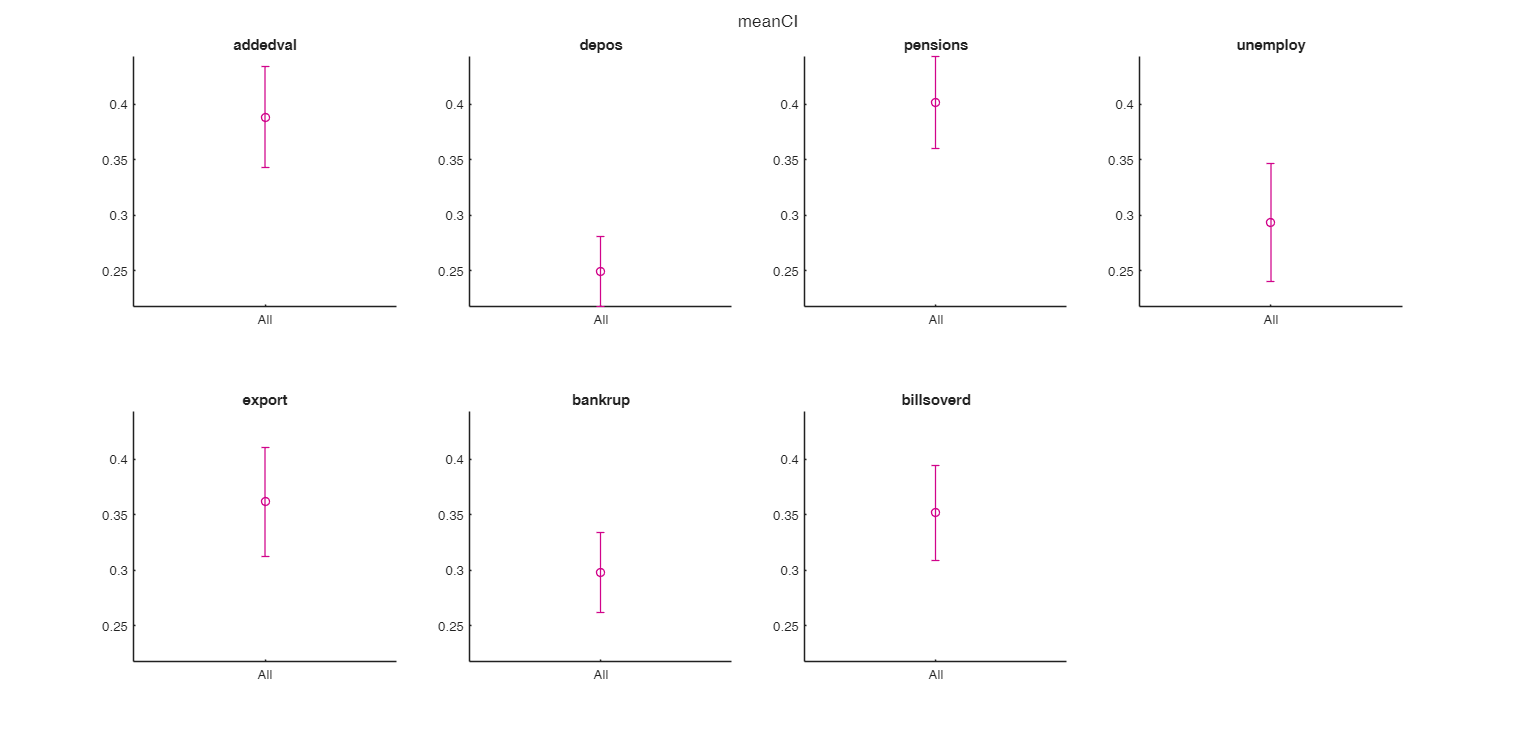
Example of option plots and no grouping variable.
Example of option plots and no grouping variable.
load citiesItaly.mat
% rescale all the variables in the interval [0 1];
CIT=normalize(citiesItaly,"range");
figure
lab=CIT.Properties.VariableNames;
boxchart(CIT,lab)
xticklabels(lab)
title('Boxplots of normalized data in [0 1]')
figure
grpstatsFS(CIT,[],["meanci" "mean" "median"],'plots',1);
disp("Note that the confidence intervals for variables 2 and 6 are much lower")
disp("than the others due to the presence of outlying observations")
Note that the confidence intervals for variables 2 and 6 are much lower than the others due to the presence of outlying observations