FSM
FSM computes forward search estimator in multivariate analysis
Description
Examples
 FSM with all default options.
FSM with all default options.
n=200;
v=3;
randn('state', 123456);
Y=randn(n,v);
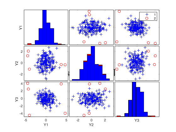
% Contaminated data
Ycont=Y; Ycont(1:5,[1,3]) = Ycont(1:5,[1,3])+sign(randn(5,2))*4.5;
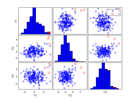
[out]=FSM(Ycont);
title('Outliers detected by FSM','Fontsize',24,'Interpreter','LaTex');
Warning: Using 'state' to set RANDN's internal state causes RAND, RANDI, and
RANDN to use legacy random number generators. This syntax is not recommended.
See <a href="matlab:helpview([docroot '\techdoc\math\math.map'],'update_random_number_generator')">Replace Discouraged Syntaxes of rand and randn</a> to use RNG to replace the
old syntax.
-------------------------
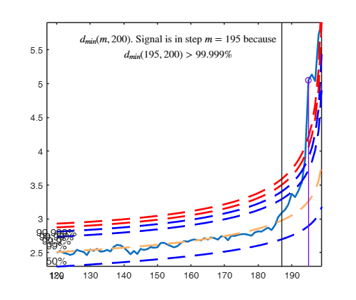
Signal detection loop
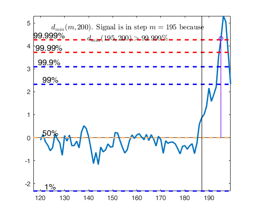
dmin(195,200)>99.9% and dmin(196,200)>99.9% and rmin(194,200)>99%
drmin(194,200)>99.9% and dmin(195,200)>99.9% and rmin(196,200)>99%
dmin(195,200)>99% at final step: Bonferroni signal in the final part of the search.
dmin(195,200)>99.999%
-------------------
Signal validation
Validated signal
-------------------------------
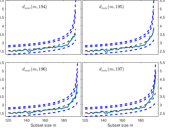
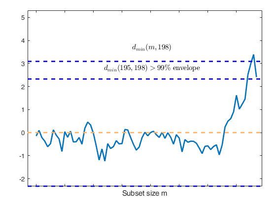
Start resuperimposing envelopes from step m=194
Superimposition stopped because d_{min}(195,196)>99% envelope
$d_{min}(195,196)>99$\% envelope
----------------------------
Final output
Number of units declared as outliers=5
Summary of the exceedances
1 99 999 9999 99999
0 6 6 4 4

FSM with optional arguments.
FSM with optional arguments.FSM with plots showing envelope superimposition.
n=200;
v=3;
randn('state', 123456);
Y=randn(n,v);
% Contaminated data
Ycont=Y;
Ycont(1:5,:)=Ycont(1:5,:)+3;
[out]=FSM(Ycont,'plots',2);
-------------------------
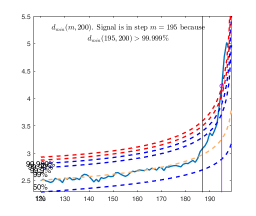
Signal detection loop
dmin(195,200)>99.9% and dmin(196,200)>99.9% and rmin(194,200)>99%
drmin(194,200)>99.9% and dmin(195,200)>99.9% and rmin(196,200)>99%
dmin(195,200)>99.999%
-------------------
Signal validation
Validated signal
-------------------------------
Start resuperimposing envelopes from step m=194
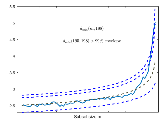
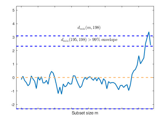
Superimposition stopped because d_{min}(195,198)>99% envelope
$d_{min}(195,198)>99$\% envelope
Subsample of 197 units is homogeneous
----------------------------
Final output
Number of units declared as outliers=3
Summary of the exceedances
1 99 999 9999 99999
0 6 5 3 3
Related Examples
FSM with plots showing envelope superimposition in normal
coordinates.
FSM with plots showing envelope superimposition in normal
coordinates.
n=200;
v=3;
randn('state', 123456);
Y=randn(n,v);
% Contaminated data
Ycont=Y;
Ycont(1:5,:)=Ycont(1:5,:)+3;
plots=struct;
plots.ncoord=1;
[out]=FSM(Ycont,'plots',plots);
-------------------------
Signal detection loop
dmin(195,200)>99.9% and dmin(196,200)>99.9% and rmin(194,200)>99%
drmin(194,200)>99.9% and dmin(195,200)>99.9% and rmin(196,200)>99%
dmin(195,200)>99.999%
-------------------
Signal validation
Validated signal
-------------------------------
Start resuperimposing envelopes from step m=194
Superimposition stopped because d_{min}(195,198)>99% envelope
$d_{min}(195,198)>99$\% envelope
Subsample of 197 units is homogeneous
----------------------------
Final output
Number of units declared as outliers=3
Summary of the exceedances
           1          99         999        9999       99999
           0           6           5           3           3

Input Arguments
Output Arguments
References
Riani, M., Atkinson, A.C. and Cerioli, A. (2009), Finding an unknown number of multivariate outliers, "Journal of the Royal Statistical Society Series B", Vol. 71, pp. 201-221.
Cerioli, A., Farcomeni, A. and Riani M. (2014), Strong consistency and robustness of the Forward Search estimator of multivariate location and scatter, "Journal of Multivariate Analysis", Vol. 126, pp. 167-183, http://dx.doi.org/10.1016/j.jmva.2013.12.010