FSMtra
FSMtra computes MLE of transformation parameters.
Description
Examples
FSMtra with all default options.
Baby food data.
load('baby.mat');
Y=baby{:,6:end};
% FS based on untrasnformed data H_0:\lambda=1 for all variables
% Plot of mle of transformation parameters with all default options
% Compare the output with Figure 4.7 p. 167 of ARC (2004)
[out]=FSMtra(Y);
 FSMtra with optional arguments.
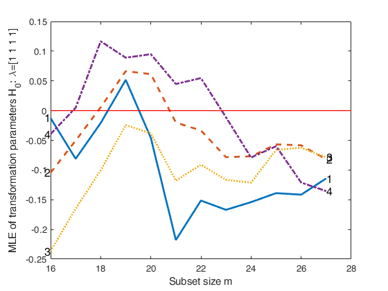
FSMtra with optional arguments.Plot the maximum likelihood estimates of the transformation parameters.
% Baby food data.
load('baby.mat');
Y=baby{:,6:end};
% FS based on untrasnformed data H_0:\lambda=1 for all variables
% Plot of mle of transformation parameters with all default options
% Compare the output with Figure 4.7 p. 167 of ARC (2004)
[out]=FSMtra(Y,'plotsmle',1);
Related Examples
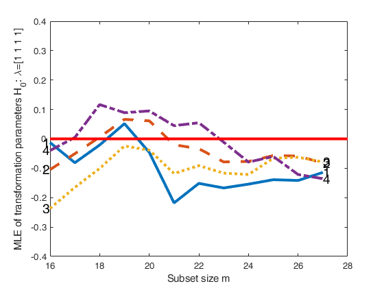
Personalized options for plotsmle.
Personalized options for plotsmle.Baby food data.
load('baby.mat');
Y=baby{:,6:end};
% Personalized options for plotsmle
plotsmle=struct;
plotsmle.LineWidth=3;
plotsmle.LineWidthEnv=3;
plotsmle.FontSize=14;
plotsmle.ylim=[-0.4 0.4];
[out]=FSMtra(Y,'plotsmle',plotsmle);
FSMtra based on log transformed data.
Baby food data.
load('baby.mat');
Y=baby{:,6:end};
% FS based on log trasnformed data H_0:\lambda=0 for all variables
% Plot of mle of transformation parameters with all default options
v=size(Y,2);
plotsmle=struct;
plotsmle.ylim=[-0.4 1];
[out]=FSMtra(Y,'la0',zeros(v,1),'init',11,'plotsmle',plotsmle);
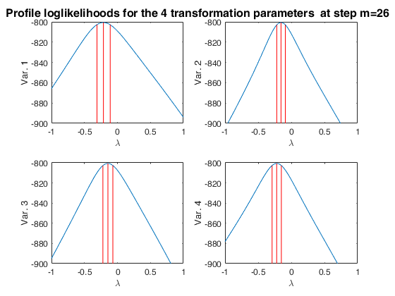
Monitoring the profile log likelihood of the transformation parameters.
Monitoring the profile log likelihood of the transformation parameters.Baby food data ignoring the regression structure.
load('baby.mat');
Y=baby{:,6:end};
% FS based on log trasnformed data H_0:\lambda=0 for all variables
% Plot of mle of transformation parameters with all default options
v=size(Y,2);
plotsmle=struct;
plotsmle.ylim=[-0.4 1];
prolik=struct;
prolik.steps=26;
prolik.xlim=[-1 1];
[out]=FSMtra(Y,'la0',zeros(v,1),'init',11,'prolik',prolik);
Swiss heads data, Example 1.
FSMtra based on untransformed data for all variables
load('head.mat');
Y=head{:,:};
[out]=FSMtra(Y,'plotsmle',1);
Swiss heads data, Example 2.
FSMtra based on untransformed data H_0:\lambda=1 for all variables
load('head.mat');
Y=head{:,:};
% Analysis of profile loglikelihoods at step m=198
prolik=struct;
prolik.steps=198;
prolik.xlim=[-3 5];
[out]=FSMtra(Y,'prolik',prolik);
Swiss heads data, Example 3.
FSMtra based on untransformed data H_0:\lambda=1 for all variables
load('head.mat');
Y=head{:,:};
% Monitoring of likelihood ratio test
% Compare the output with Figure 4.13 p. 172 of ARC (2004)
[out]=FSMtra(Y,'plotslrt',1);
Swiss heads data, Example 4.
load('head.mat');
Y=head{:,:};
% FS based on untransformed data H_0:\lambda=1 for variable 4
% Monitoring of likelihood ratio test
% Compare the output with Figure 4.14 p. 173 of ARC (2004)
[out]=FSMtra(Y,'ColToTra',4,'plotslrt',1);
Mussels data, Example 1.
FSMtra based on untransformed data H_0:\lambda=1 for all variables
load('mussels.mat');
Y=mussels{:,:};
% Compare plot of mle with Figure 4.19 p. 178 of ARC (2004)
% Compare plot of lrt with Figure 4.18 p. 178 of ARC (2004)
[out]=FSMtra(Y,'plotsmle',1,'plotslrt',1);
Mussels data, Example 2.
load('mussels.mat');
Y=mussels{:,:};
% FSMtra based on with H_0:\lambda=[1 0.5 1 0 1/3]
% Compare plot of mle with Figure 4.21 p. 178 of ARC (2004)
% Compare plot of lrt with Figure 4.20 p. 178 of ARC (2004)
[out]=FSMtra(Y,'la0',[1 0.5 1 0 1/3],'plotsmle',1,'plotslrt',1);
Swiss bank notes data, Example 1.
load('swiss_banknotes');
Y=swiss_banknotes{:,:};
n=size(Y,1);
Y1=repmat(max(Y),n,1);
Y=Y./Y1;
% FS using just one value of lambda for all the variables
% Compare plot of lrt with left panel of Figure 4.69 p. 225 of ARC (2004)
[out]=FSMtra(Y,'init',40,'onelambda',1,'plotslrt',1);
Swiss bank notes data, Example 2.
load('swiss_banknotes');
Y=swiss_banknotes{:,:};
n=size(Y,1);
Y1=repmat(max(Y),n,1);
Y=Y./Y1;
% FS using just one value of lambda for all the variables
% Search starts with the first 20 genuine notes
% Compare plot of lrt with central panel of Figure 4.69 p. 225 of ARC (2004)
[out]=FSMtra(Y,'init',20,'onelambda',1,'bsb',1:20,'plotslrt',1);
Swiss bank notes data, Example 3.
load('swiss_banknotes');
Y=swiss_banknotes{:,:};
Y=Y(1:100,:);
% FS using just one value of lambda for all the variables
% Monitoring of mle of lambda (Figure 4.66 p. 223 of ARC (2004))
% Monitoring of lrt (Figure 4.67 p. 223 of ARC (2004))
plotsmle=struct;
plotsmle.ylim=[-1.5 2.5];
% Profile loglikelihoods at steps m=90 and m=100
% (Figure 4.68 p. 224 of ARC (2004))
prolik=struct;
prolik.steps=[90 100];
prolik.xlim=[-3.2 3.2];
[out]=FSMtra(Y,'onelambda',1,'plotsmle',plotsmle,'plotslrt',1,'prolik',prolik);
Swiss bank notes data, Example 4.
load('swiss_banknotes');
Y=swiss_banknotes{:,:};
n=size(Y,1);
Y1=repmat(max(Y),n,1);
Y=Y./Y1;
% FS using just one value of lambda for all the variables
% Search starts with the first 20 forged notes
% Compare plot of lrt with right panel of Figure 4.69 p. 225 of ARC (2004)
[out]=FSMtra(Y,'init',20,'onelambda',1,'bsb',101:120,'plotslrt',1);
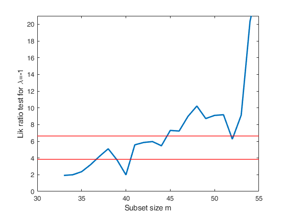
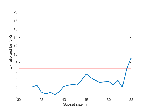
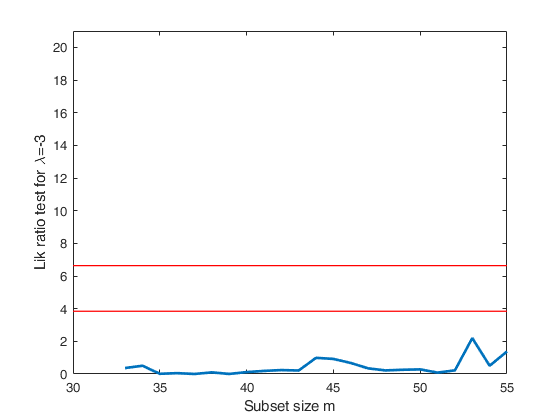
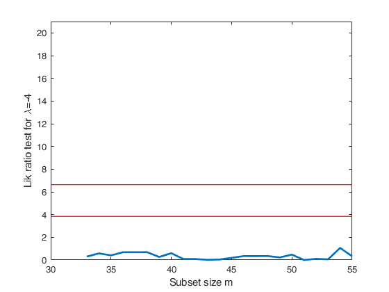
Track records data.
Track records data.
load('recordfg');
Y=recordfg{:,:};
n=size(Y,1);
Y1=repmat(max(Y),n,1);
Y=Y./Y1;
la0=[-1 -2 -3 -4];
tags={'lrt-1' 'lrt-2' 'lrt-3' 'lrt-4'};
plotslrt=struct;
plotslrt.ylim=[0 21];
ii=1;
for la=la0;
plotslrt.Tag=tags{ii};
[out]=FSMtra(Y,'plotslrt',plotslrt,'onelambda',1,'la0',la);
ii=ii+1;
end
disp(out)
% Compare these 4 plots with Figure 4.50 p. 207 of ARC (2004)
    MLEtra: [23×2 double]
    Exflag: [23×2 double]
    LIKrat: [23×2 double]
        Un: [22×11 double]
     class: 'FSMtra'
Emilia Romagna data, Example 1.
load('emilia2001')
Y=emilia2001{:,:};
% Replace zeros with min values for variables specified in sel
sel=[6 10 12 13 19 21];
for i=sel
Y(Y(:,i)==0,i)=min(Y(Y(:,i)>0,i));
end
% Extract demographic variables
Y1=Y(:,[1 2 3 4 5 10 11 12 13]);
colnames={'1' '2' '3' '4' '5' '10' '11' '12' '13'};
[out]=FSMtra(Y1,'plotsmle',1,'colnames',colnames);
% Compare the plot with Figure 4.31 p. 188 of ARC (2004)
Emilia Romagna data, Example 2.
Yeo and Johnson family of transformations is used. In this case there is no need to correct 0 values
load('emilia2001')
Y=emilia2001{:,:};
% Extract demographic variables
Y1=Y(:,[1 2 3 4 5 10 11 12 13]);
colnames={'1' '2' '3' '4' '5' '10' '11' '12' '13'};
plotslrt=struct;
plotslrt.ylim=[-8.2 8.2];
ColToComp=[1 3 5 9];
la0=[0 0.25 0 0.5 0.5 0 0 0.5 0.25];
[out]=FSMfan(Y1,la0,'ColToComp',ColToComp,'plotslrt',plotslrt,'colnames',colnames,'family','YJ');
Emilia Romagna data, Example 3.
Demographic data
load('emilia2001')
Y=emilia2001{:,:};
% Replace zeros with min values for variables specified in sel
sel=[6 10 12 13 19 21];
for i=sel
Y(Y(:,i)==0,i)=min(Y(Y(:,i)>0,i));
end
% Extract demographic variables
Y1=Y(:,[1 2 3 4 5 10 11 12 13]);
colnames={'1' '2' '3' '4' '5' '10' '11' '12' '13'};
la0=[0 0.25 0 0.5 0.5 0 0 0.5 0.25];
prolik=struct;
prolik.steps=[331];
prolik.xlim=[-1 1];
plotslrt=struct;
plotslrt.ylim=[4 21];
[out]=FSMtra(Y1,'plotsmle',1,'plotslrt',plotslrt,'la0',la0,'colnames',colnames,'prolik',prolik);
% Compare the plots with Figures 4.32, 4.33 and 4.34 p. 189-191 of ARC (2004)
Emilia Romagna data, Example 4.
Modified wealth variables.
load('emilia2001')
Y=emilia2001{:,:};
% Replace zeros with min values for variables specified in sel
sel=[6 10 12 13 19 21];
for i=sel
Y(Y(:,i)==0,i)=min(Y(Y(:,i)>0,i));
end
% Modify wealth variables
Y(:,16)=100-Y(:,16);
Y(:,23)=100-Y(:,23);
% Extract wealth variables
Y1=Y(:,[14:23]);
colnames={'14' '15' '16' '17' '18' '19' '20' '21' '22' '23'};
la0=[0 1 0.25 1 1 0.5 -0.5 0.25 0.25 -1];
[out]=FSMtra(Y1,'plotslrt',1,'la0',la0,'colnames',colnames);
% Compare the plot with left panel of Figure 4.38 p. 188 of ARC (2004)
Emilia Romagna data, Example 5.
Modified wealth variables.
load('emilia2001')
Y=emilia2001{:,:};
% Replace zeros with min values for variables specified in sel
sel=[6 10 12 13 19 21];
for i=sel
Y(Y(:,i)==0,i)=min(Y(Y(:,i)>0,i));
end
% Modify wealth variables
Y(:,16)=100-Y(:,16);
Y(:,23)=100-Y(:,23);
% Extract wealth variables
Y1=Y(:,[14:23]);
colnames={'14' '15' '16' '17' '18' '19' '20' '21' '22' '23'};
la0=[0.5 1 0.25 1 1 0.5 -0.5 0.25 0.25 -1];
[out]=FSMtra(Y1,'plotslrt',1,'la0',la0,'colnames',colnames);
% Compare the plot with Figure 4.40 p. 196 of ARC (2004)
Emilia Romagna data, Example 6.
Work variables.
load('emilia2001')
Y=emilia2001{:,:};
% Replace zeros with min values for variables specified in sel
sel=[6 10 12 13 19 21 25 26];
for i=sel
Y(Y(:,i)==0,i)=min(Y(Y(:,i)>0,i));
end
% Extract work variables
Y1=Y(:,[6:9 24:28]);
colnames={'6' '7' '8' '9' '24' '25' '26' '27' '28'};
la0=[0.25,0,2,-1,0,1.5,0.5,1,1];
[out]=FSMtra(Y1,'plotsmle',1,'plotslrt',1,'la0',la0,'colnames',colnames);
% Compare the plots with Figures 4.41 p. 197 and left panel of Figure
% 4.42 of ARC (2004)
Emilia Romagna data, Example 7.
Modified work variables.
load('emilia2001')
Y=emilia2001{:,:};
% Replace zeros with min values for variables specified in sel
sel=[6 10 12 13 19 21];
for i=sel
Y(Y(:,i)==0,i)=min(Y(Y(:,i)>0,i));
end
% Modify variables 25 and 26
Y(:,25)=100-Y(:,25);
Y(:,26)=100-Y(:,26);
% Extract work variables
Y1=Y(:,[6:9 24:28]);
colnames={'6' '7' '8' '9' '24' '25' '26' '27' '28'};
la0=[0.25,0,2,-1,0,0,1.5,1,1];
[out]=FSMtra(Y1,'plotsmle',1,'plotslrt',1,'la0',la0,'colnames',colnames);
Input Arguments
Y — Input data.
Matrix.
n x v data matrix; n observations and v variables. Rows of Y represent observations, and columns represent variables.
Missing values (NaN's) and infinite values (Inf's) are allowed, since observations (rows) with missing or infinite values are automatically excluded from the computations.
Data Types: single|double
Name-Value Pair Arguments
Specify optional comma-separated pairs of Name,Value arguments.
Name is the argument name and Value
is the corresponding value. Name must appear
inside single quotes (' ').
You can specify several name and value pair arguments in any order as
Name1,Value1,...,NameN,ValueN.
 'family','YJ'
, 'init',50
, 'bsb',[4 6 9]
, 'rf',0.99
, 'ColToTra',[1 3]
, 'la0',[-1 0]
, 'onelambda',0
,'optmin.Display','off'
,'speed',0
,'colnames', {'1' '2' '3' '4' '5' '10' '11' '12' '13'};
,'prolik',7
,'plotsmle',1
,'plotslrt',1
,'msg',1
family
—parametric transformation to use.string.
String which identifies the family of transformations which must be used. Character. Possible values are 'BoxCox' (default) or 'YJ'.
The Box-Cox family of power transformations equals (y^{\lambda}-1)/\lambda for \lambda not equal to zero, and \log(y) if \lambda = 0.
The Yeo-Johnson (YJ) transformation is the Box-Cox transformation of y+1 for nonnegative values, and of |y|+1 with parameter 2-lambda for y negative.
The basic power transformation returns y^{\lambda} if \lambda is not zero, and \log(\lambda) otherwise.
Remark. BoxCox and the basic power family can be used just if input y is positive. Yeo-Johnson family of transformations does not have this limitation.
Example: 'family','YJ'
Data Types: char
init
—Beginning of monitoring.scalar.
Scalar which defines where to start monitoring required diagnostics.
Note that if bsb is suppliedinit>=length(bsb). If init is not specified it will be set equal to floor(n*0.6).
Example: 'init',50
Data Types: double
bsb
—Units forming initial subset.vector.
It contains the units forming initial subset. The default value of bsb is '' that is the initial subset is found through the intersection of robust bivariate ellipses This option is useful if a forced start is required.
Example: 'bsb',[4 6 9]
Data Types: double
rf
—confidence level for bivariate ellipses.scalar.
Default is 0.9. If bsb is not empty this argument is ignored.
Example: 'rf',0.99
Data Types: double
ColToTra
—Variables to transform.vector.
Vector which specifies the variables which must be transformed. Vector. It is a k x 1 integer vector.
Example: 'ColToTra',[1 3]
Data Types: double
la0
—Values of transformation parameters.vector.
Vector which contains set of transformation parameters for the k ColtoTra. It is a k-by-1 vector. The ordering of Mahalanobis distances at each step of the forward search uses variables transformed with la0.
la0 empty is equivalent to its default value la0=ones(length(ColToTra),1).
Example: 'la0',[-1 0]
Data Types: double
onelambda
—common value of lambda.scalar.
If onelambda=1, a common value lambda is estimated for all variables specified in ColToTra.
Example: 'onelambda',0
Data Types: double
optmin
—Optimation options.structure.
It contains the options dealing with the maximization algorithm. Use optimset to set these options. Notice that the maximization algorithm which is used is fminunc is the optimization toolbox is present else is fminsearch.
Example: 'optmin.Display','off'
Data Types: double
speed
—Start with previous values in the maximization procedure.scalar.
If speed=1 the initial value at step m of the maximization procedure is the final value at step m-1 else it is la0. Default value 1. The maximization procedure is fminunc or fminsearch.
Example: 'speed',0
Data Types: double
colnames
—variable names.cell array of strings.
It contains the names of the variables of the dataset. Cell array of strings of length v. If colnames is empty then the sequence 1:v is created to label the variables.
Example: 'colnames', {'1' '2' '3' '4' '5' '10' '11' '12' '13'};
Data Types: cell array of strings
prolik
—Monitor profile log likelihood.scalar | structure.
It specifies whether it is necessary to monitor the profile log likelihood of the transformation parameters at selected steps of the search.
If prolik is a scalar, the plot of the profile loglikelihoods is produced at step m=n with all default parameters.
If prolik is a structure it may contain the following fields:
| Value | Description |
|---|---|
steps |
vector containing the steps of the fwd search for which profile logliks have to be plotted. The default value of steps is n; |
clev |
scalar between 0 and 1 determining confidence level for each element of lambda based on the asymptotic chi1^2 of twice the loglikelihood ratio. The default confidence level is 0.95; |
xlim |
vector with two elements determining minimum and maximum values of lambda in the plots of profile loglikelihoods. The default value of xlim is [-2 2]; |
LineWidth |
line width of the vertical lines defining confidence levels of the transformation parameters. |
Example: 'prolik',7
Data Types: double
plotsmle
—plot mle.scalar | structure.
It specifies whether it is necessary to plot the maximum likelihood estimates of the transformation parameters. Three horizontal lines associated respectively with values -1, 0 and 1 are added to the plot.
If prolik is a scalar, the plot of the monitoring of maximum likelihood estimates of transformation parameters is produced on the screen with all the default options.
If plotsmle is a structure, it may contain the following fields:
| Value | Description |
|---|---|
xlim |
minimum and maximum on the x axis; |
ylim |
minimum and maximum on the y axis; |
LineWidth |
Line width of the trajectories of mle of transformation parameters; |
LineStyle |
cell containing Line styles of the trajectories of mle of transformation parameters; |
LineWidthEnv |
Line width of the horizontal lines; |
Tag |
tag of the plot (default is pl_mle); |
FontSize |
font size of the text labels which identify the trajectories. |
Example: 'plotsmle',1
Data Types: double
plotslrt
—plot lrt.scalar | structure.
It specifies whether it is necessary to plot the likelihood ratio test.
If plotslrt is a scalar, the plot of the monitoring of likelihood ratio test is produced on the screen with all default options.
If plotslrt is a strucure, it may contain the following fields:
| Value | Description |
|---|---|
xlim |
minimum and maximum on the x axis; |
ylim |
minimum and maximum on the y axis; |
LineWidth |
Line width of the trajectory of lrt of transformation parameters; |
conflev |
vector which defines the confidence levels of the horizontal line for the likelihood ratio test (default is conflev=[0.95 0.99]); |
LineWidthEnv |
Line width of the horizontal lines; |
Tag |
tag of the plot (default is pl_lrt). |
Example: 'plotslrt',1
Data Types: double
msg
—Level of display on the screen.scalar.
It controls whether to display or not messages about great interchange on the screen. If msg==1 (default) messages are displayed on the screen else no message is displayed on the screen.
Example: 'msg',1
Data Types: double
Output Arguments
out — description
Structure
Structure which contains the following fields
| Value | Description |
|---|---|
MLEtra |
n-init+1 x v matrix which contains the monitoring of MLE of transformation parameters: 1st col = fwd search index (from init to n); 2nd col = MLE of variable 1; 3rd col = MLE of variable 2; ...; (v+1)th col = MLE of variable v. |
LIKrat |
n-init+1 x 2 = matrix which contains the monitoring of likelihood ratio for testing H0:\lambda=la0: 1st col = fwd search index (from init to n); 2nd col = value of the likelihood ratio. |
Exflag |
n-init+1 x 2 = matrix which contains the monitoring of the integer identifying the reason why the maximization algorithm terminated. See help page fminunc of the optimization toolbox for the list of values of exitflag and the corresponding reasons the algorithm terminated: 1st col = fwd search index (from init to n); 2nd col = the value that describes the exit condition |
Un |
(n-init) x 11 Matrix which contains the unit(s) included in the subset at each step of the fwd search. REMARK: in every step the new subset is compared with the old subset. Un contains the unit(s) present in the new subset but not in the old one Un(1,2) for example contains the unit included in step init+1 Un(end,2) contains the units included in the final step of the search |
class |
'FSMtra'; |
References
Atkinson, A.C., Riani, M. and Cerioli, A. (2004), "Exploring multivariate data with the forward search", Springer Verlag, New York.