FSRms

FSRms performs robust model selection using flexible trimming in linear regression

Syntax

Description

example

outms =FSRms(y, X) FSRms with all default options.

example

outms =FSRms(y, X, Name, Value) FSRms with optional arguments.

Examples

expand all

  • FSRms with all default options.
  • Common part to all examples: load Ozone dataset, tranform the response using logs and add a time trend.

    X=load('ozone.txt');
    X(:,end)=log(X(:,end));
    X=[(-40:39)' X];
    y=X(:,end);
    X=X(:,1:end-1);
    [Cpms]=FSRms(y,X);

  • FSRms with optional arguments.
  • Perform robust model selection and show the generalized candlestick plot.

    X=load('ozone.txt');
    X(:,end)=log(X(:,end));
    X=[(-40:39)' X];
    y=X(:,end);
    X=X(:,1:end-1);
    labels={'Time','1','2','3','4','5','6','7','8'};
    [Cpms]=FSRms(y,X,'labels',labels,'plots',1);
    small p=9
    small p=8
    small p=7
    small p=6
    small p=5
    small p=4
    Warning: Rank deficient, rank = 2, tol =  8.881784e-12. 
    Warning: Rank deficient, rank = 2, tol =  1.241267e-11. 
    Warning: Rank deficient, rank = 2, tol =  1.631688e-11. 
    ------------------------------
    Warning: Number of subsets without full rank equal to 10.3%
    small p=3
    
    Click here for the graphical output of this example (link to Ro.S.A. website).

    Related Examples

    expand all

  • Reproduce the candlestick plot given in Figure 5 of Riani and Atkinson (2010).
  • X=load('ozone.txt');
    X(:,end)=log(X(:,end));
    X=[(-40:39)' X];
    y=X(:,end);
    X=X(:,1:end-1);
    labels={'Time','1','2','3','4','5','6','7','8'};
    n=length(y);
    fin_step=floor([n*0.1 n*0.02]);
    outms=FSRms(y,X,'fin_step',fin_step,'plots',1,'labels',labels,'smallpint',[4:7]);
    %The figure has slightly changed and certainly there can be some random
    %fluctuations due to the number of subset which have been used to initialize
    %the search for each model. However, The indication of the previous two
    %Figures does not change at all: the values of smallp of 4 or 5 should yield
    %a satisfactory model. For smallp = 4 the best model has the trend, x3 and
    %x7, although the plot shows the values of Cp(m) increasing towards the end
    %of the search. By far the most stable model for smallp= 5 adds x2 to these
    %variables.
    small p=7
    small p=6
    small p=5
    small p=4
    
    Click here for the graphical output of this example (link to Ro.S.A. website)

  • Considering all submodels.
  • Perform robust model selection and show the generalized candlestick plot considering all submodels for each smallp from 2 to size(X).

    X=load('ozone.txt');
    X(:,end)=log(X(:,end));
    X=[(-40:39)' X];
    y=X(:,end);
    X=X(:,1:end-1);
    labels={'Time','1','2','3','4','5','6','7','8'};
    [Cpms]=FSRms(y,X,'labels',labels,'ignore',0,'plots',1);

  • Comparing results of different settings.
  • Perform robust model selection and show the generalized candlestick plot. Restric attention to the models with size in the interval 4:6 Compare the results using ignore=1 with those with ignore=0 default option ignore=1.

    X=load('ozone.txt');
    X(:,end)=log(X(:,end));
    X=[(-40:39)' X];
    y=X(:,end);
    X=X(:,1:end-1);
    labels={'Time','1','2','3','4','5','6','7','8'};
    [Cpms]=FSRms(y,X,'smallpint',4:6,'labels',labels,'plots',1);
    % ignore=0
    [Cpms]=FSRms(y,X,'ignore',0,'smallpint',4:6,'labels',labels,'plots',1);
    % with ignore=0 but changing the threshold for excluding models
    [Cpms]=FSRms(y,X,'smallpint',4:6,'labels',labels,'plots',1,'ExclThresh',0.99999999999999);
    small p=6
    small p=5
    small p=4
    small p=6
    small p=5
    Warning: Rank deficient, rank = 3, tol =  1.112200e-11. 
    Warning: Rank deficient, rank = 3, tol =  1.355801e-11. 
    Warning: Rank deficient, rank = 3, tol =  1.583108e-11. 
    Warning: Rank deficient, rank = 3, tol =  1.810506e-11. 
    small p=4
    small p=6
    small p=5
    small p=4
    
    Click here for the graphical output of this example (link to Ro.S.A. website)

  • Changing confidence bands.
  • Same options as before but using different confidence bands.

    X=load('ozone.txt');
    X(:,end)=log(X(:,end));
    X=[(-40:39)' X];
    y=X(:,end);
    X=X(:,1:end-1);
    labels={'Time','1','2','3','4','5','6','7','8'};
    qu=[0.01 0.5 0.99];
    [Cpms]=FSRms(y,X,'smallpint',4:6,'labels',labels,'plots',1,'quant',qu);

  • Personalized LineWidth and CandleWidth.
  • X=load('ozone.txt');
    X(:,end)=log(X(:,end));
    X=[(-40:39)' X];
    y=X(:,end);
    X=X(:,1:end-1);
    labels={'Time','1','2','3','4','5','6','7','8'};
    LineWidth=2;
    CandleWidth=0.03;
    [Cpms]=FSRms(y,X,'smallpint',4:6,'labels',labels,'plots',1,'LineWidth',LineWidth,'CandleWidth',CandleWidth);

  • Input fin_step supplied as fraction (1).
  • For example when fin_step=[0.3 0.1] the central part of the search goes from m=round(n*0.7)=56 to m=round(n*0.9)=72 and the final part of the search goes from m=73 to m=80.

    X=load('ozone.txt');
    X(:,end)=log(X(:,end));
    X=[(-40:39)' X];
    y=X(:,end);
    X=X(:,1:end-1);
    labels={'Time','1','2','3','4','5','6','7','8'};
    [Cpms]=FSRms(y,X,'smallpint',4:6,'labels',labels,'plots',1,'fin_step',[0.3 0.1]);

  • Input fin_step supplied as fraction (2).
  • For example when fin_step=[0.36 0.06] the central part of the search goes from m=round(n*0.64)=51 to m=round(n*0.94)=75 and the final part of the search goes from m=76 to m=80.

    X=load('ozone.txt');
    X(:,end)=log(X(:,end));
    X=[(-40:39)' X];
    y=X(:,end);
    X=X(:,1:end-1);
    labels={'Time','1','2','3','4','5','6','7','8'};
    [Cpms]=FSRms(y,X,'smallpint',4:6,'labels',labels,'plots',1,'fin_step',[0.36 0.06]);

  • Input fin_step supplied as integers.
  • For example when fin_step=[20 5] the central part of the search goes from m=n-20=61 to m=n-5=75 and the final part of the search goes from m=76 to m=80.

    % It is worthwhile to notice that independently on how fin_step is
    % chosen, the message of the generalized candlestick plot remains the
    % same. In other words, the best two models with 5 variables are always
    % (Time,4,5,6) and (Time,2,4,5)
    % while two reasonable models with 6 variables are (Time,2,4,5,6) and
    % (Time,2,3,4,5).
    X=load('ozone.txt');
    X(:,end)=log(X(:,end));
    X=[(-40:39)' X];
    y=X(:,end);
    X=X(:,1:end-1);
    labels={'Time','1','2','3','4','5','6','7','8'};
    [Cpms]=FSRms(y,X,'smallpint',4:6,'labels',labels,'plots',1,'fin_step',[25 5], 'CandleWidth',0.01);

    Input Arguments

    expand all

    y — Response variable. Vector.

    A vector with n elements that contains the response variables.

    Missing values (NaN's) and infinite values (Inf's) are allowed, since observations (rows) with missing or infinite values will automatically be excluded from the computations.

    Data Types: single| double

    X — Predictor variables. Matrix.

    Data matrix of explanatory variables (also called 'regressors') of dimension (n x (bigP-1)).

    The intercept will be added in automatic way, so that the dimension of the full model is bigP Rows of X represent observations, and columns represent variables. Missing values (NaN's) and infinite values (Inf's) are allowed, since observations (rows) with missing or infinite values will automatically be excluded from the computations.

    Data Types: single| double

    Name-Value Pair Arguments

    Specify optional comma-separated pairs of Name,Value arguments. Name is the argument name and Value is the corresponding value. Name must appear inside single quotes (' '). You can specify several name and value pair arguments in any order as Name1,Value1,...,NameN,ValueN.

    Example: 'intercept',false , 'init',100 starts monitoring from step m=100 , 'h',round(n*0,75) , 'nsamp',1000 , 'lms',1 , 'nocheck',true , 'smallpint',3 , 'labels',{'1','2'} , 'fin_step',[1 50] , 'first_k',5 , 'ignore',1 , 'ExclThresh',0.9 , 'meanmed',1 , 'plots',1 , 'rl',0.3 , 'quant',[0.01;0.99] , 'CandleWidth',0.01 , 'LineWidth',0.01 , 'ylimy',[0 10] , 'xlimy',[0 10]

    intercept —Indicator for constant term.true (default) | false.

    Indicator for the constant term (intercept) in the fit, specified as the comma-separated pair consisting of 'Intercept' and either true to include or false to remove the constant term from the model.

    Example: 'intercept',false

    Data Types: boolean

    init —Search initialization.scalar.

    It specifies the initial subset size to start monitoring the required quantities, if init is not specified it set equal to: p+1, if the sample size is smaller than 40;

    min(3*p+1,floor(0.5*(n+p+1))), otherwise.

    Example: 'init',100 starts monitoring from step m=100

    Data Types: double

    h —The number of observations that have determined the least trimmed squares estimator.scalar.

    h is an integer greater or equal than [(n+p+1)/2] but smaller then n

    Example: 'h',round(n*0,75)

    Data Types: double

    nsamp —Number of subsamples which will be extracted to find the robust estimator.scalar.

    Number of subsamples which will be extracted to find the robust estimator. If nsamp=0 all subsets will be extracted.

    They will be (n choose smallp).

    Remark. if the number of all possible subset is <1000 the default is to extract all subsets otherwise just 1000.

    Example: 'nsamp',1000

    Data Types: double

    lms —Criterion to use to find the initlal subset to initialize the search.scalar.

    If lms=1 (default) Least Median of Squares is computed, else Least Trimmed of Squares is computed.

    Example: 'lms',1

    Data Types: double

    nocheck —Check input arguments.boolean.

    If nocheck is equal to true no check is performed on matrix y and matrix X. Note that y and X are left unchanged. In other words the additional column of ones for the intercept is not added. As default nocheck=false.

    Example: 'nocheck',true

    Data Types: boolean

    smallpint —submodels to consider.vector.

    It specifies which submodels (number of variables) must be considered.

    The default is to consider all models from size 2 to size bigP-1. In other words, as default, smallpint=(bigP-1):-1:2.

    When smallpint=2 all submodels including one explanatory variable and the constant will be considered.

    When smallpint=3 all submodels including two explanatory variables and a constant will be considered. ....

    Example: 'smallpint',3

    Data Types: double

    labels —names of the explanatory variables.cell array of strings.

    Cell array of strings of length bigP-1 containing the names of the explanatory variables.

    If labels is a missing value the following sequence of strings will be automatically created for labelling the column of matrix X (1,2,3,4,5,6,7,8,9,A,B,C,D,E,E,G,H,I,J,K,...,Z)

    Example: 'labels',{'1','2'}

    Data Types: cell

    fin_step —Initial and final step.vector with two elements.

    Initial and final step of the search which has to be monitored to choose the best models as specified in scalar first_k.

    The first element of the vector specifies the initial step of the search which has to be monitored to choose the best models as specified in scalar first_k below. The second element specifies the ending point of the central part of the search. This information will be used to create the 
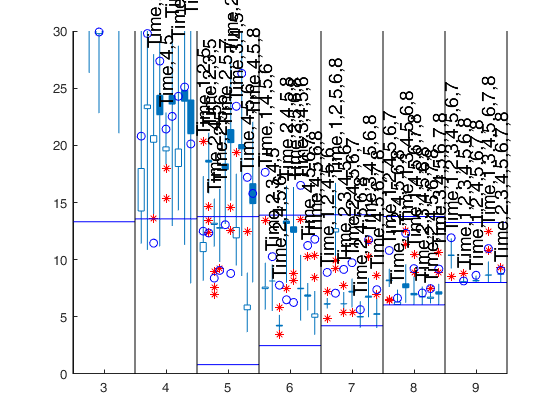
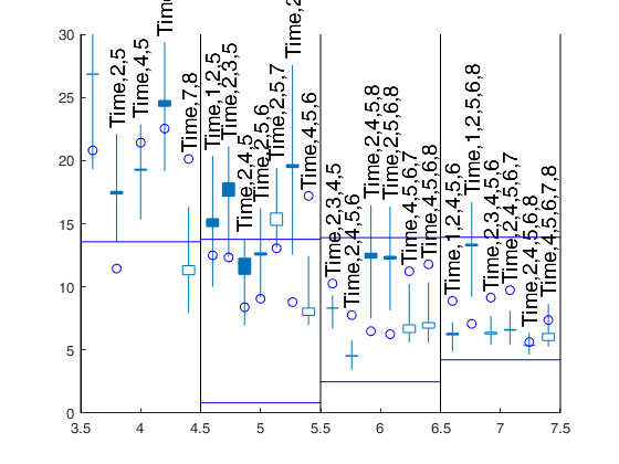
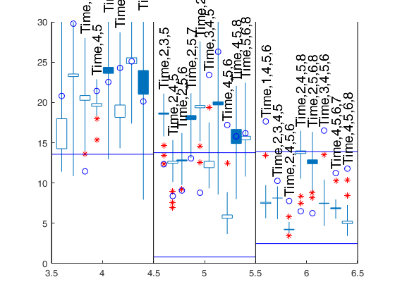
candlestick Cp plot.

    If the elements of fin_step are integers greater or equal 1 they refer to the number of steps. For example if fin_step=[10 3] the program considers the last 10 steps to choose the best models and the central part of the search is defined up to step n-3.

    If the elements of fin_step are real numbers alpha (0<alpha<0.5) in the interval (0 0.5] then the program considers the last round(n*alpha) steps.

    As default fin_step(1)=round(n*0.2) that is the last 20% of the steps are considered.

    As default fin_step(2)=round(n*0.05) that is the central part of the search extends up to 95% of the observations

    Example: 'fin_step',[1 50]

    Data Types: double

    first_k —Number of models to consider.scalar.

    Number of best models to consider in each of the last fin_step.

    For example if first_k=5 in each of the fin_step the models which had the 5 smallest values of Cp are considered. As default first_k=3

    Example: 'first_k',5

    Data Types: double

    ignore —submodels to consider.scalar.

    If ignore=1, when dealing with p explanatory variables, the submodels of the models with p+1 explanatory variables which were considered irrelevant according to option ExclThresh, are not considered. As default ignore=1, because this saves computational time.

    If ignore is different from 1, for each p all submodels of size p which contain a constant are considered

    Example: 'ignore',1

    Data Types: double

    ExclThresh —Exclusion threshold.scalar.

    It has effect only if ignore=1.

    Exclusion threshold associated to the uppper percentage point of the F distribution of Cp which defines the threshold for each p declaring models as irrelevant.

    The default value of ExclThresh is 0.99999 that is the models whose minimum value of Cp in the part of the search defined by fin_step is above ExclThresh are stored for each p. If option ignore=1, the submodels with p-1 explanatory variables which are contained inside the models considered irrelevant are not considered

    Example: 'ExclThresh',0.9

    Data Types: double

    meanmed —Boxes of tha candles.scalar.

    It specifies how to construct the boxes of the candles.

    If meanmed=1 boxes are constructed using mean and median else using the first and third quartile.

    Example: 'meanmed',1

    Data Types: double

    plots —Plot on the screen.scalar.

    If plot==1 a candlestick Cp plot is created on the screen else (default) no plot is shown on the screen The options below only work when plots=1

    Example: 'plots',1

    Data Types: double

    rl —spread of the candles around each integer value defining the size of the submodels.scalar.

    For example if rl=0.4 for each smallp candles are spread in the interval [smallp-rl smallp+rl]. The default value of rl is 0.4. rl does not have to be greater than 0.45 otherwise the candles overlap

    Example: 'rl',0.3

    Data Types: double

    quant —quantiles for the horizontal lines associated with the confidence bands of Cp.vector.

    The default is to plot 2.5% and 97.5% envelopes. In other words the default is quant=[0.025;0.975];

    Example: 'quant',[0.01;0.99]

    Data Types: double

    CandleWidth —width of the boxes associated with the central part of the search.scalar.

    The default width is 0.05;

    Example: 'CandleWidth',0.01

    Data Types: double

    LineWidth —Line Width (in points) for the vertical lines outside the boxes of the candles.scalar.

    The default LineWidth is 0.5 points.

    Example: 'LineWidth',0.01

    Data Types: double

    ylimy —minimum and maximum on the y axis.vector.

    Default value is [-2 50] (automatic scale)

    Example: 'ylimy',[0 10]

    Data Types: double

    xlimx —minimum and maximum on the x axis.vector.

    Default value is '' (automatic scale)

    Example: 'xlimy',[0 10]

    Data Types: double

    Output Arguments

    expand all

    outms — description Structure

    Structure which contains the following fields

    Value Description
    stor

    k x 9 matrix containing statistics which can be used to create the candles 1st col: max Cp values;

    2nd col: min Cp values;

    3rd col: average Cp values;

    4nd col: median Cp values;

    Remark: the information in the first 4 columns is referred to the central part of the search.

    5th col: x coordinates (or size of submodel);

    6th col: number of explanatory variables of the submodel 7th col: y coordinate of final Cp;

    8th col: units entering the final step of the search;

    9th col: maximum Cp value during the (central and final part of the) search (This information is used to print the labels on top of each model).

    outl

    r x 4 matrix containing information about 'influential units' or empty matrix.

    Influential units in this context are defined as the units which enter the subset in the final part of the search and bring the value of Cp below the minimum or above the maximum value of the central part of the search.

    1st col: x coordinates;

    2nd col: y coordinates;

    3rd col: step of entry into subset;

    4nd col: unit number.

    If matrix outl contains more columns they are ignored.

    siz

    vector of length 2 containing information about n (number of units of the sample and bigP, number of explanatory variables, including the constant, in the full model). This information is necessary to compute the envelopes.

    MAL

    (n-init+1) x (k+1) matrix Mallows Cp monitored along the search for the selected models.

    1st col is fwd search index;

    2nd col is associated with first selected model;

    3rd col is associated with second selected model;

    ............;

    (k+1)th col is associated with k-th selected model Notice that k<=(n choose smallp) and that all models contain the constant.

    LAB

    cell array of strings of length k containing the labels of the models which have been extracted. First element of LAB is associated with second column of matrix MAL ... last element of LAB is associated with last column of matrix MAL

    Remark: the loop through all values of smallp works backwards in the sense that first all possible submodels of size bigP-1 are considered, then the models with size bigP-2 ...

    References

    Riani M. and Atkinson A.C. (2010), Robust Model Selection with Flexible Trimming, "Computational Statistics and Data Analysis", Vol. 54, p. 3300-3312.

    See Also

    |

    This page has been automatically generated by our routine publishFS