GUIregress
GUIregress shows the necessary calculations to obtain simple linear regression statistics in a GUI.
Description
Examples
 Calculation of unweighted regression.
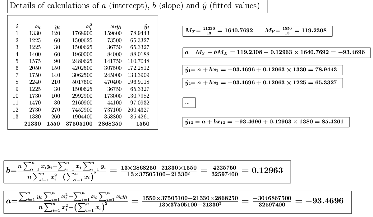
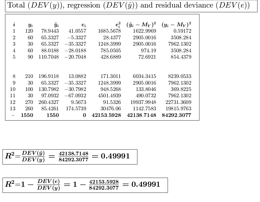
Calculation of unweighted regression.In this example we know the monthly income of 13 families and we estimate the correlation with the free time expenditure. (See page 223 of [MRZ]).
% x= monthly income of 13 families.
% y= free time expenditure.
x=[1330 1225 1225 1400 1575 2050 1750 2240 1225 1730 1470 2730 1380];
y=[120 60 30 60 90 150 140 210 30 100 30 270 260];
out=GUIregress(x,y);
Use of option plots.
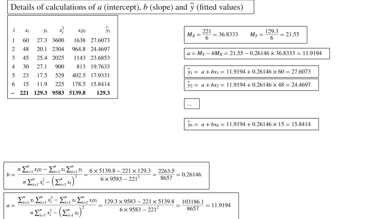
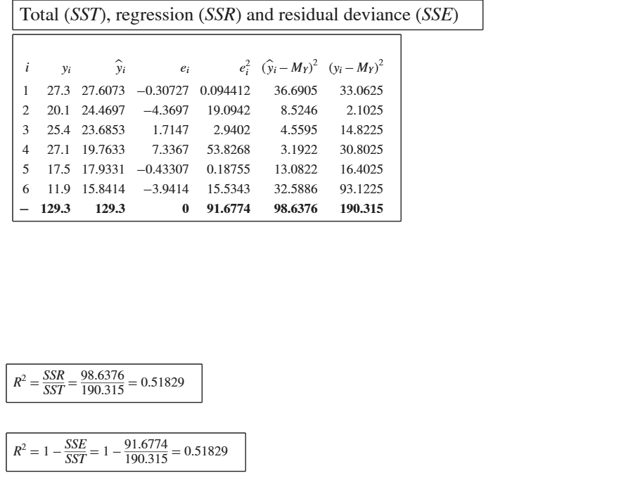
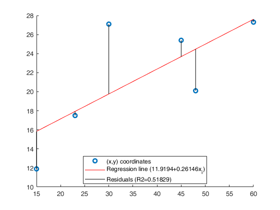
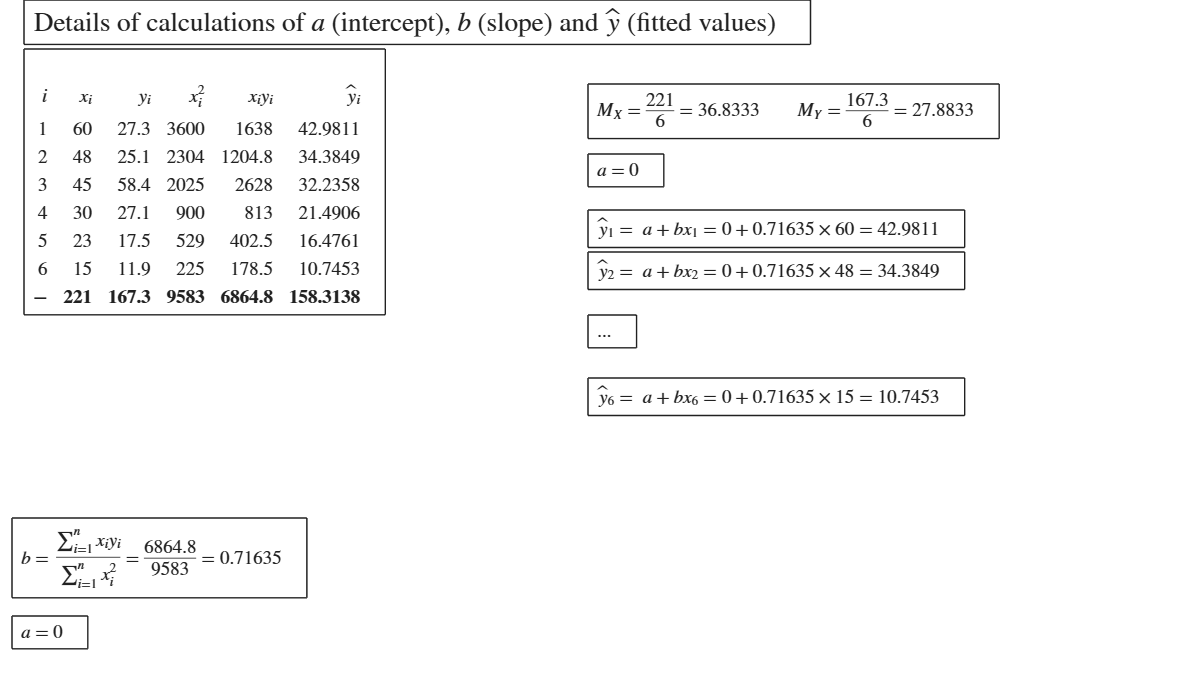
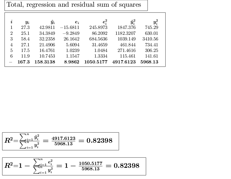
Use of option plots.The following data matrix reports, for 6 countries, the tourism revenues (y) recorded in a given year (in billions of dollars) and the number of foreign visitors (x) in the same year (in millions of units). (See page 101 of [CMR])
x=[60 48 45 30 23 15];
y=[27.3 20.1 25.4 27.1 17.5 11.9];
out=GUIregress(x,y,'plots',true);
ans =

  Legend ((x,y) coordinates, Regression line (11.9194+0.26146x…) with properties:

         String: {1×3 cell}
       Location: 'best'
    Orientation: 'vertical'
       FontSize: 9.00
       Position: [0.57 0.40 0.29 0.09]
          Units: 'normalized'

  Use GET to show all properties
Related Examples
Use of option intercept.
Use of option intercept.The following data matrix reports, for 6 countries, the tourism revenues (y) recorded in a given year (in billions of dollars) and the number of foreign visitors (x) in the same year (in millions of units). (See page 101 of [CMR])
x=[60 48 45 30 23 15];
y=[27.3 25.1 58.4 27.1 17.5 11.9];
out=GUIregress(x,y,'intercept',false,'plots',false);

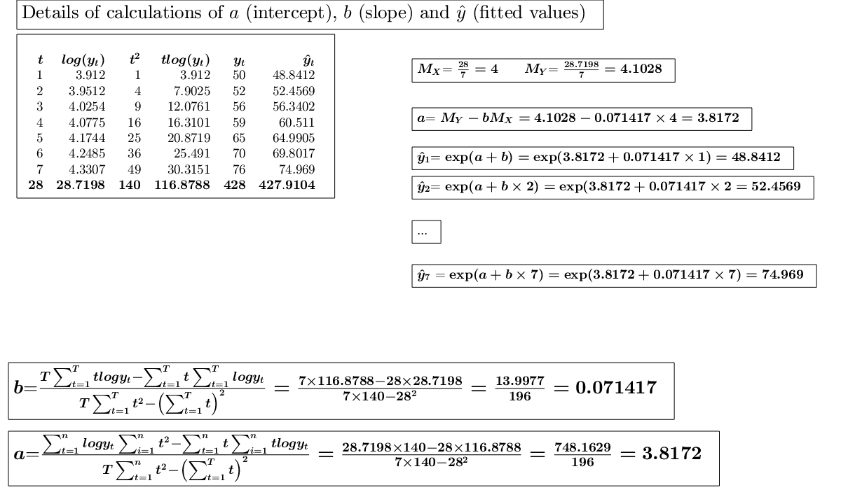
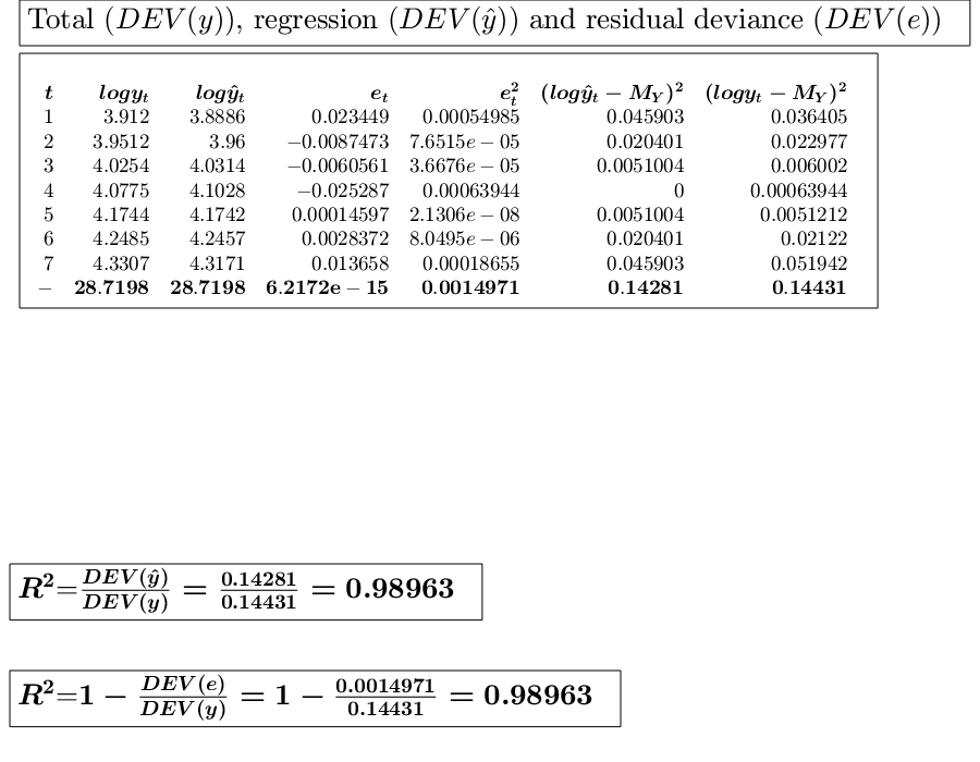
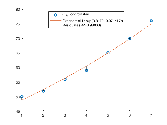
Example of exponential interpolation.
Example of exponential interpolation.The values of a company's production, in millions of euros were as follows: (See page 116 of [CMR])
x=1:7;
y=[50 52 56 59 65 70 76];
% Analyze the trend of the company's production using an exponential fit.
out=GUIregress([],y,'interpolant','exponential','plots',true,'timeseries', true);
ans =

  Legend ((t,y_t) coordinates, Exponential fit exp(3.8172+0.07…) with properties:

         String: {1×3 cell}
       Location: 'best'
    Orientation: 'vertical'
       FontSize: 9.00
       Position: [0.56 0.27 0.30 0.09]
          Units: 'normalized'

  Use GET to show all properties
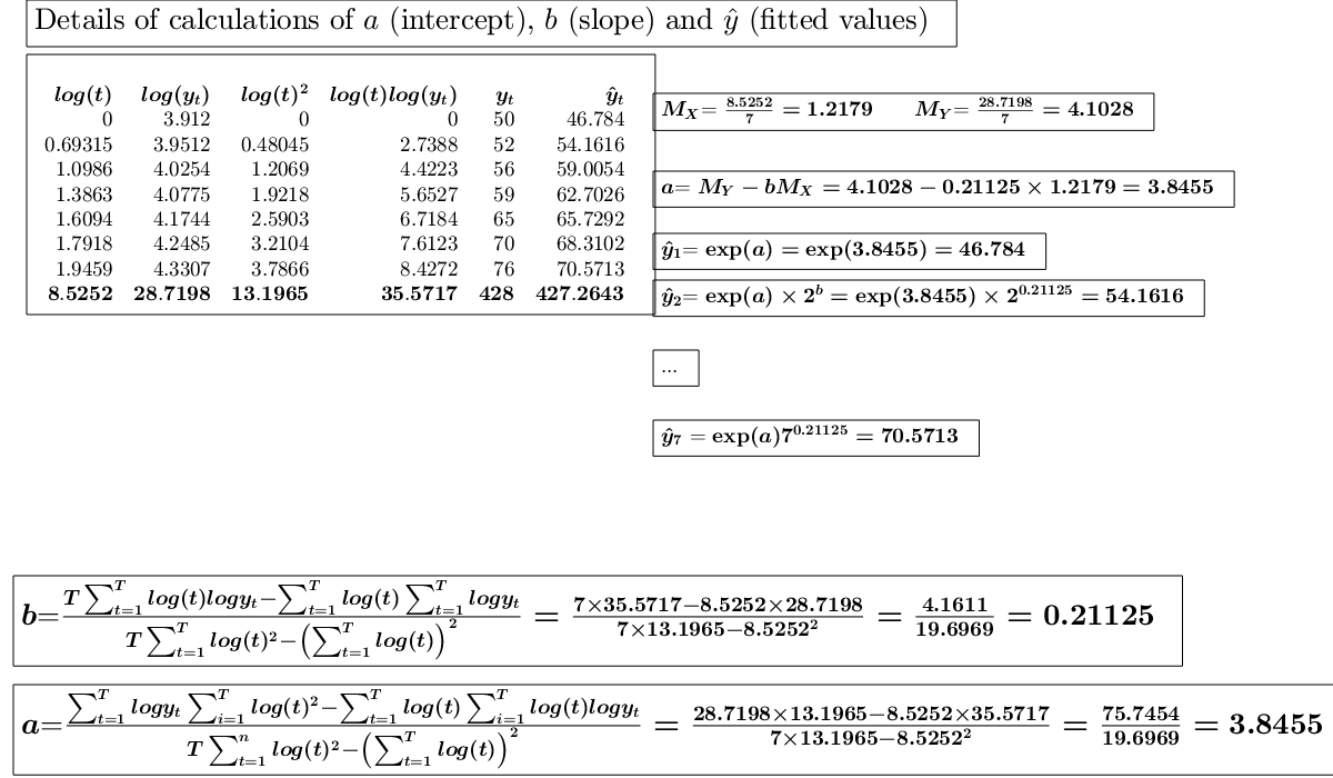
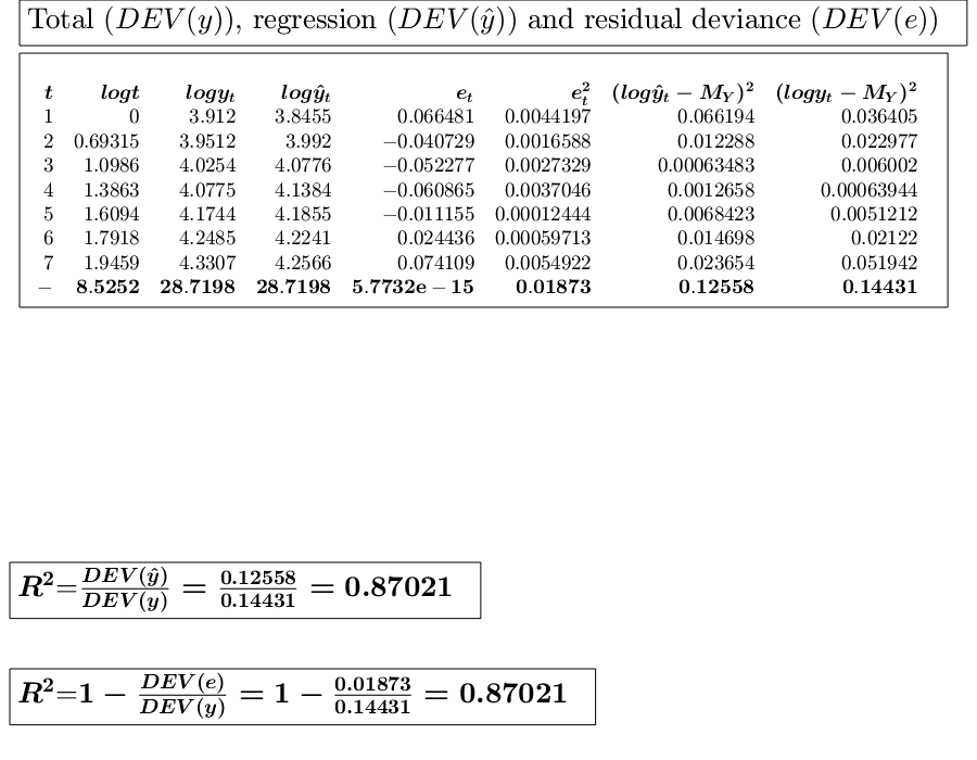
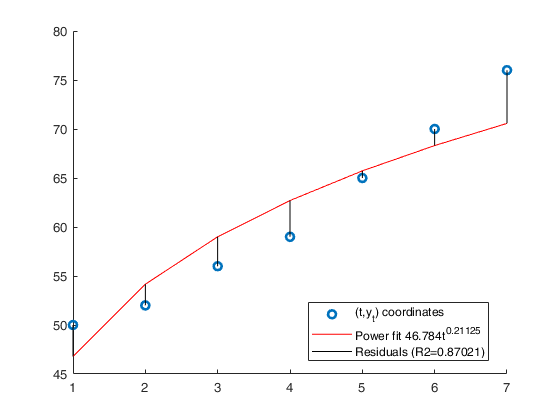
Example of power interpolation.
Example of power interpolation.The values of a company's production, in millions of euros were as follows: (See page 116 of [CMR])
x=1:7;
y=[50 52 56 59 65 70 76];
% Analyze the trend of the company's production using a power fit.
out=GUIregress(x,y,'interpolant','power','plots',true,'timeseries', true);
ans =

  Legend ((t,y_t) coordinates, Power fit 46.784t^{0.21125}, Re…) with properties:

         String: {1×3 cell}
       Location: 'best'
    Orientation: 'vertical'
       FontSize: 9.00
       Position: [0.15 0.81 0.21 0.10]
          Units: 'normalized'

  Use GET to show all properties

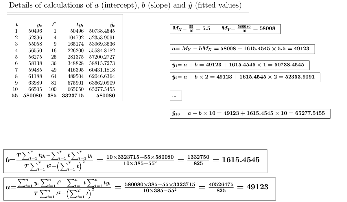
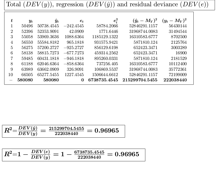
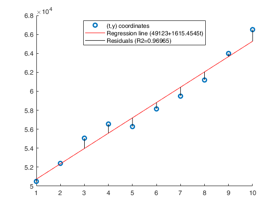
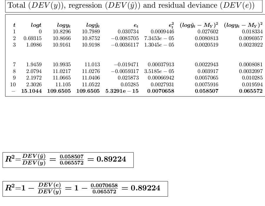
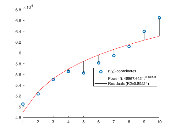
Example of linear, exponential and power interpolation.
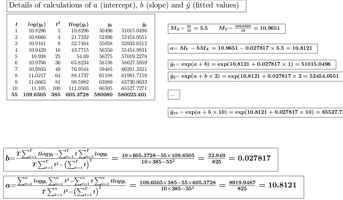
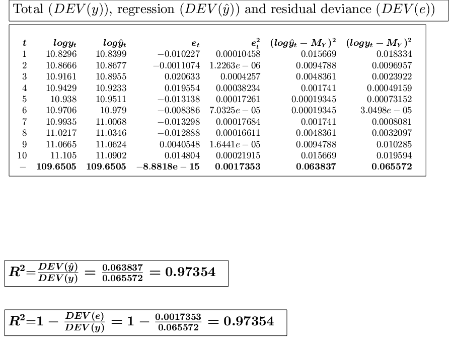
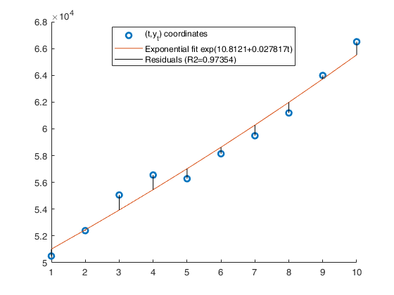
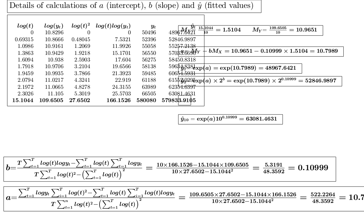
Example of linear, exponential and power interpolation.Time series of the value of a commodity, in euros were as follows: (See page 269 of [MRZ])
y=[50496 52396 55058 56550 56275 58138 59485 61188 63989 66505];
x=1:10;
% Analyze the trend of the company's production using a linear fit.
out=GUIregress(x,y,'interpolant','linear','plots',true, 'timeseries', true);
% Analyze the trend of the company's production using an exponential fit.
out=GUIregress(x,y,'interpolant','exponential','plots',true,'timeseries',true);
% Analyze the trend of the company's production using an power fit.
out=GUIregress(x,y,'interpolant','power','plots',true,'timeseries',true)
ans =

  Legend ((t,y) coordinates, Regression line (49123+1615.4545t…) with properties:

         String: {1×3 cell}
       Location: 'best'
    Orientation: 'vertical'
       FontSize: 9.00
       Position: [0.57 0.36 0.29 0.09]
          Units: 'normalized'

  Use GET to show all properties


ans =

  Legend ((t,y_t) coordinates, Exponential fit exp(10.8121+0.0…) with properties:

         String: {1×3 cell}
       Location: 'best'
    Orientation: 'vertical'
       FontSize: 9.00
       Position: [0.56 0.27 0.30 0.09]
          Units: 'normalized'

  Use GET to show all properties


ans =

  Legend ((t,y_t) coordinates, Power fit 48967.6421t^{0.10999}…) with properties:

         String: {1×3 cell}
       Location: 'best'
    Orientation: 'vertical'
       FontSize: 9.00
       Position: [0.66 0.13 0.23 0.10]
          Units: 'normalized'

  Use GET to show all properties


out =

  struct with fields:

    tabledata: [11×6 table]
         expa: 10.80
            a: 48967.64
            b: 0.11
           R2: 0.89
           ta: 480.54
           tb: 8.14
     confinta: []
     confintb: []

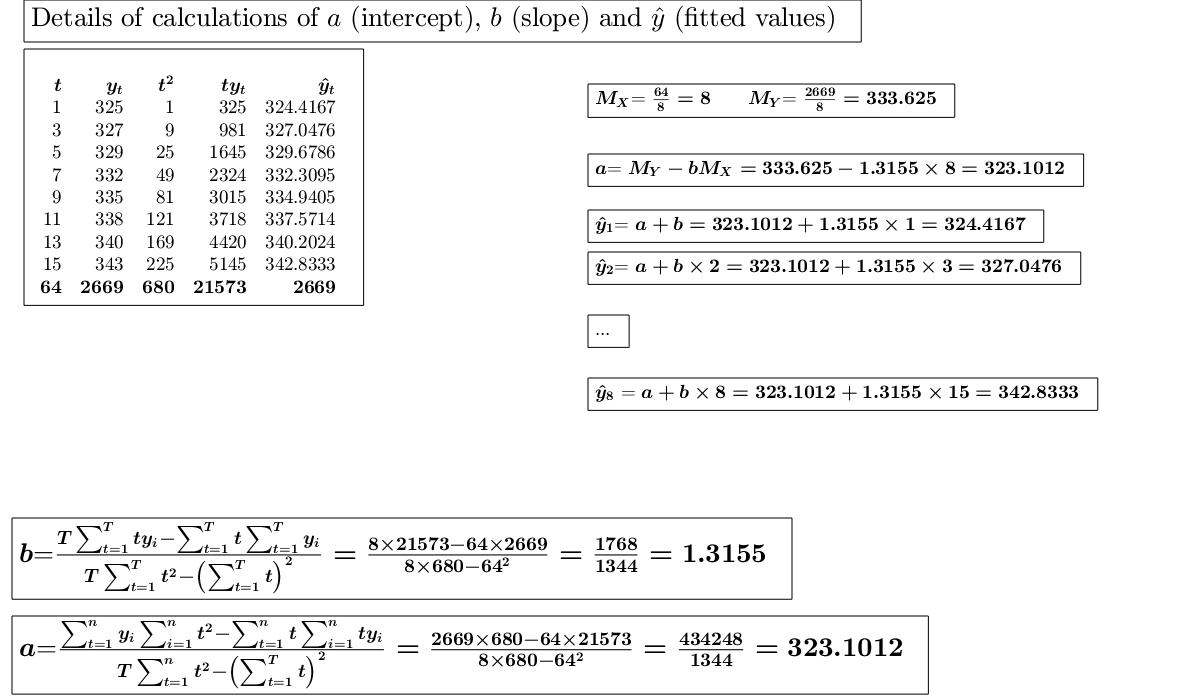
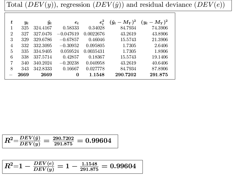
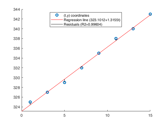
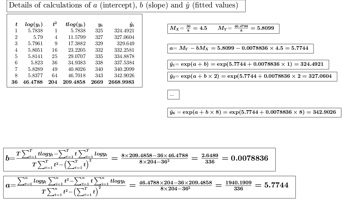
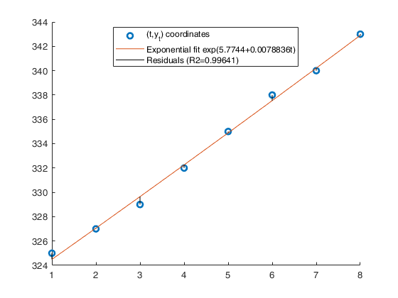
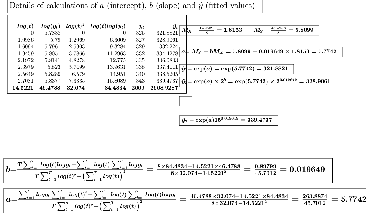
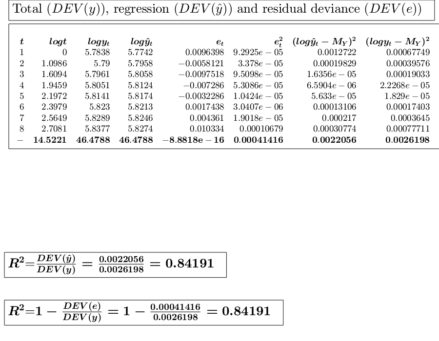
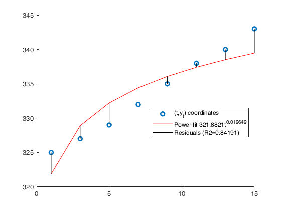
Example of linear and power interpolation.
Example of linear and power interpolation.
close all
% Time series....,  (See ex 4.26 of [CMR])
xb=1:8;
xa=[1 3 5 7 9 11 13 15];
y=[325 327 329 332 335 338 340 343];
% Analyze the trend of the company's production using a linear fit.
out=GUIregress(xa,y,'interpolant','linear','plots',true, 'timeseries', true);
% Analyze the trend of the company's production using an exponential fit.
out=GUIregress(xb,y,'interpolant','exponential','plots',true, 'timeseries', true);
% Analyze the trend of the company's production using a power fit.
out=GUIregress(xa,y,'interpolant','power','plots',true, 'timeseries', true);
ans =

  Legend ((t,y) coordinates, Regression line (323.1012+1.3155t…) with properties:

         String: {1×3 cell}
       Location: 'best'
    Orientation: 'vertical'
       FontSize: 9.00
       Position: [0.57 0.36 0.28 0.09]
          Units: 'normalized'

  Use GET to show all properties


ans =

  Legend ((t,y_t) coordinates, Exponential fit exp(5.7744+0.00…) with properties:

         String: {1×3 cell}
       Location: 'best'
    Orientation: 'vertical'
       FontSize: 9.00
       Position: [0.56 0.40 0.30 0.09]
          Units: 'normalized'

  Use GET to show all properties


ans =

  Legend ((t,y_t) coordinates, Power fit 321.8821t^{0.019649},…) with properties:

         String: {1×3 cell}
       Location: 'best'
    Orientation: 'vertical'
       FontSize: 9.00
       Position: [0.66 0.13 0.22 0.10]
          Units: 'normalized'

  Use GET to show all properties
Use of option inferential.
Use of option inferential.In a survey on pollution, we want to verify whether the content of a certain pollutant in the air, expressed in micrograms per cubic meter (Y) is linked to the number of manufacturing companies with more than 20 employees (X). The results obtained in some cities are given below:
x=[91 453 254 412 334 428 341 125];
y=[13 12 17 56 29 35 49 27];
out=GUIregress(x,y,'inferential',0.90,'plots',false);
% There is not enough evidence to state that is not 0 in the population
% and the estimated relationship between the two variables is
% significant. The value of the linear index of determination
% (R2=0.159) shows a very poor fit of the regression line. The
% estimated model is therefore of no use for interpreting the causes of
% pollution.
Input Arguments
Output Arguments
References
Milioli, M.A., Riani, M., Zani, S. (2019), "Introduzione all'analisi dei dati statistici (Quarta edizione ampliata)". [MRZ]
Cerioli, A., Milioli, M.A., Riani, M. (2016), "Esercizi di statistica (Quinta edizione)". [CMR]
See Also
GUIvar
|
GUImad
|
GUIskewness