TBwei
TBwei computes weight function psi(u)/u for Tukey's biweight
Syntax
w=TBwei(u,c)example
Examples
Related Examples
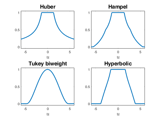
 Compare four different weight functions.
Compare four different weight functions.Initialize graphical parameters.
FontSize=14;
x=-6:0.01:6;
ylim1=-0.05;
ylim2=1.05;
xlim1=min(x);
xlim2=max(x);
LineWidth=2;
subplot(2,2,1)
ceff095HU=HUeff(0.95,1);
weiHU=HUwei(x,ceff095HU);
plot(x,weiHU,'LineWidth',LineWidth)
xlabel('$u$','Interpreter','Latex','FontSize',FontSize)
title('Huber','FontSize',FontSize)
ylim([ylim1 ylim2])
xlim([xlim1 xlim2])
subplot(2,2,2)
ceff095HA=HAeff(0.95,1);
weiHA=HAwei(x,ceff095HA);
plot(x,weiHA,'LineWidth',LineWidth)
xlabel('$u$','Interpreter','Latex','FontSize',FontSize)
title('Hampel','FontSize',FontSize)
ylim([ylim1 ylim2])
xlim([xlim1 xlim2])
subplot(2,2,3)
ceff095TB=TBeff(0.95,1);
weiTB=TBwei(x,ceff095TB);
plot(x,weiTB,'LineWidth',LineWidth)
xlabel('$u$','Interpreter','Latex','FontSize',FontSize)
title('Tukey biweight','FontSize',FontSize)
ylim([ylim1 ylim2])
xlim([xlim1 xlim2])
subplot(2,2,4)
ceff095HYP=HYPeff(0.95,1);
ktuning=4.5;
weiHYP=HYPwei(x,[ceff095HYP,ktuning]);
plot(x,weiHYP,'LineWidth',LineWidth)
xlabel('$u$','Interpreter','Latex','FontSize',FontSize)
title('Hyperbolic','FontSize',FontSize)
ylim([ylim1 ylim2])
xlim([xlim1 xlim2])
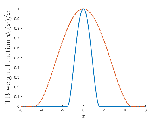
Compare two weight functions for 2 different values of c.
Compare two weight functions for 2 different values of c.In the first we fix the bdp (value of efficiency is automatically given), while in the second we find the efficiency (the value of bdp is automatically given).
close all
x=-6:0.01:6;
lwd=2;
hold('on')
c=TBbdp(0.5,1);
rhoTB=TBwei(x,c);
plot(x,rhoTB,'LineStyle','-','LineWidth',lwd)
c=TBeff(0.95,1);
rhoTB=TBwei(x,c);
plot(x,rhoTB,'LineStyle','-.','LineWidth',lwd)
xlabel('$x$','Interpreter','Latex','FontSize',16)
ylabel('TB weight function $\psi_c(x)/x$','Interpreter','Latex','FontSize',20)
Input Arguments
Output Arguments
More About
References
Maronna, R.A., Martin D. and Yohai V.J. (2006), "Robust Statistics, Theory and Methods", Wiley, New York.
Riani, M., Cerioli, A. and Torti, F. (2014), On consistency factors and efficiency of robust S-estimators, "TEST", Vol. 23, pp. 356-387.