boxcoxR
boxcoxR finds MLE of lambda in linear regression (and confidence interval) using Box Cox, YJ or extended YJ transformation
Description
The function computes the profile log Likelihood for a range of values of the transformation parameter (lambda) and computes the MLE of lambda in the supplied range. Supported families are Box Cox, Yeo and Johnson and extended Yeo and Johnson (Atkinson et al. 2020).
The profile log-likelihood is computed as:
where y(\lambda) is the vector of transformed observations using Box Cox family, Yeo and Johnson or extended Yao and Johnson family \beta(\lambda) = (X'X)^{-1} X' y(\lambda) and J is the Jacobian of the transformation.
boxcoxR using YJ transformation.out
=boxcoxR(y,
X,
Name, Value)
Examples
 boxcoxR with all default options.
boxcoxR with all default options.Use the wool data.
load('wool.txt','wool');
y=wool(:,4);
X=wool(:,1:3);
out=boxcoxR(y,X);
disp(['Estimate of lambda using Box Cox is =',num2str(out.lahat)])
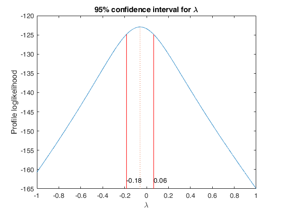
Estimate of lambda using Box Cox is =-0.059
boxcoxR using YJ transformation.
boxcoxR using YJ transformation.
load('wool.txt','wool');
y=wool(:,4);
X=wool(:,1:3);
out=boxcoxR(y,X,'family','YJ');
disp(['Estimate of lambda using YJ family is =',num2str(out.lahat)])
Estimate of lambda using YJ family is =-0.062
Related Examples
Example of use of option plots combined with laseq.
Example of use of option plots combined with laseq.
load('wool.txt','wool');
y=wool(:,4);
X=wool(:,1:3);
% Plot the profile loglikelihood in the interval [-1 1]
laseq=[-1:0.0001:1];
out=boxcoxR(y,X,'plots',1,'laseq',laseq);
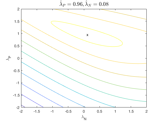
Example of use of option family.
Example of use of option family.
close all
YY=load('fondi_large.txt');
y=YY(:,2);
X=YY(:,[1 3]);
out=boxcoxR(y,X,'family','YJpn','plots',1);
% The contour plot suggests that while positive observations do not
% have to be transformed, negative observations have to be transformed using
% lambda=0. For more details see Atkinson Riani and Corbellini (2020)
Example of the use of option usefmin.
Example of the use of option usefmin.
rng(500)
% Generate regression data
outsim=simulateLM(100,'R2',0.95);
yori = outsim.y;
X = outsim.X;
% Transform in a different way positive and negative values
laPos=0.2;
laNeg=0.8;
y=normYJpn(yori,[],[laPos laNeg],'inverse',true);
% Use solver to find MLE of laPos and laNeg
usefmin=struct;
% specify maximum number of iterations
usefmin.MaxIter=100;
% Function boxcoxR initializes the optimization routine with the value
% of lambda from the last call of the optimization routine. This trick
% is very useful during the forward search when we use in step m+1 as
% initial guess of laP and laN the final estimate of laP and laN in
% step m.
% The instruction below clear persistent variables in function boxcoxR
clear boxcoxR
out=boxcoxR(y,X,'family','YJpn','plots',1,'usefmin',usefmin);
disp('MLE of laPos and laNeg')
disp(out.lahat)
MLE of laPos and laNeg
    0.2364    0.8265
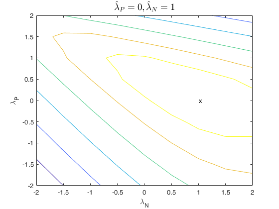
Another example of the use of option usefmin.
Another example of the use of option usefmin.In this example we specify as solver to use fminunc
rng(1000)
% Generate regression data
outsim=simulateLM(100,'R2',0.6);
yori = outsim.y;
X = outsim.X;
% Transform in a different way positive and negative values
laPos=0.4;
laNeg=-0.9;
y=normYJpn(yori,[],[laPos laNeg],'inverse',true);
% Use solver to find MLE of laPos and laNeg
usefmin=struct;
% specify maximum number of iterations
usefmin.MaxIter=100;
% Note that to specify as solver fminunc the optimization toolbox is
% needed.
usefmin.solver='fminunc';
out=boxcoxR(y,X,'family','YJpn','plots',1,'usefmin',usefmin);
disp('MLE of laPos and laNeg')
disp(out.lahat)
% Check that the values after the optimization are as expected
assert(max(abs(out.lahat-[0.3166   -0.8825]))<1e-4,'Wrong values of laP and laN')
MLE of laPos and laNeg
    0.3166   -0.8825
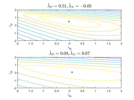
Example using simulated contaminated data.
Example using simulated contaminated data.
rng(10000)
% Generate X and y data
n=200;
X=randn(n,3);
beta=[ 1; 1; 1];
sig=0.5;
ytrue=X*beta+sig*randn(n,1);
% Contaminate response
ycont=ytrue;
ycont(21:40)=ycont(21:40)+4;
% Use two different values for laP and laN
lapos=0.5;
laneg=0;
ytra=normYJpn(ytrue,[],[lapos laneg],'inverse',true,'Jacobian',false);
yconttra=normYJpn(ycont,[],[lapos laneg],'inverse',true,'Jacobian',false);
% In this example the true values of laP and laN are 0.5 and 0 however due
% to contamination the MLE of lambda laP because very close to 0.
% This wrongly suggests a unique value of lambda.
subplot(2,1,1)
out=boxcoxR(ytra,X,'family','YJpn','plots',1);
subplot(2,1,2)
outcont=boxcoxR(yconttra,X,'family','YJpn','plots',1);
Input Arguments
Output Arguments
References
Atkinson, A.C. and Riani, M. (2000), "Robust Diagnostic Regression Analysis", Springer Verlag, New York. [see pp. 83-84]
Box, G.E.P. and Cox, D.R. (1964), An analysis of transformations (with Discussion), "Journal of the Royal Statistical Society Series B", Vol. 26, pp. 211-252.
Yeo, I.K and Johnson, R. (2000), A new family of power transformations to improve normality or symmetry, "Biometrika", Vol. 87, pp. 954-959.
Atkinson, A.C., Riani, M. and Corbellini C. (2019), The Analysis of Transformations for Profit and Loss Data, "Journal of the Royal Statistical Society. Series C: Applied Statistics", https://doi.org/10.1111/rssc.12389 [ARC]
Atkinson, A.C. Riani, M. and Corbellini A. (2021), The Box–Cox Transformation: Review and Extensions, "Statistical Science", Vol. 36, pp. 239-255, https://doi.org/10.1214/20-STS778
Acknowledgements
This function has been inspired by submission https://www.mathworks.com/matlabcentral/fileexchange/10419-box-cox-power-transformation-for-linear-models in the file exchange written by Hovav Dror, hovav@hotmail.com, March 2006