
|
FSRenvmdr |
FSRH |
 |
FSRfan
FSRfan monitors the values of the score test statistic for each lambda
Description
The transformations for negative and positive responses were determined by Yeo and Johnson (2000) by imposing the smoothness condition that the second derivative of zYJ(λ) with respect to y be smooth at y = 0.
However,some authors, for example Weisberg (2005), query the physical interpretability of this constraint, which is often violated in data analysis. Accordingly, Atkinson et al (2019) and (2020) extend the Yeo-Johnson transformation to allow two values of the transformations parameter: \lambda_N for negative observations and \lambda_P for non-negative ones.
FSRfan monitors: 1) the t test associated with the constructed variable computed assuming the same transformation parameter for positive and negative observations fixed. In short we call this test, "global score test for positive observations".
2) the t test associated with the constructed variable computed assuming a different transformation for positive observations keeping the value of the transformation parameter for negative observations fixed. In short we call this test, "test for positive observations".
3) the t test associated with the constructed variable computed assuming a different transformation for negative observations keeping the value of the transformation parameter for positive observations fixed. In short we call this test, "test for negative observations".
4) the F test for the joint presence of the two constructed variables described in points 2) and 3.
4) the F likelihood ratio test based on the MLE of \lambda_P and \lambda_N. In this case, the residual sum of squares of the null model based on a single transformation parameter \lambda is compared with the residual sum of squares of the model based on data transformed data using MLE of \lambda_P and \lambda_N.
FSRfan with optional arguments.out
=FSRfan(y,
X,
Name, Value)
Examples
 FSRfan with all default options.
FSRfan with all default options.Store values of the score test statistic for the five most common values of \lambda.
% Produce also a fan plot and display it on the screen.
% Common part to all examples: load wool dataset.
XX=load('wool.txt');
y=XX(:,end);
X=XX(:,1:end-1);
% Function FSRfan stores the score test statistic.
% In this case we use the five most common values of lambda are considered
[out]=FSRfan(y,X);
fanplotFS(out);
%The fan plot shows the log transformation is diffused throughout the data and does not depend on the presence of particular observations.
Total estimated time to complete LMS:  0.01 seconds
------------------------------
Warning: Number of subsets without full rank equal to 15.7%
Total estimated time to complete LMS:  0.00 seconds
------------------------------
Warning: Number of subsets without full rank equal to 15.7%
Total estimated time to complete LMS:  0.00 seconds
------------------------------
Warning: Number of subsets without full rank equal to 15.7%
Total estimated time to complete LMS:  0.00 seconds
------------------------------
Warning: Number of subsets without full rank equal to 15.7%
Total estimated time to complete LMS:  0.00 seconds
------------------------------
Warning: Number of subsets without full rank equal to 15.7%
Related Examples
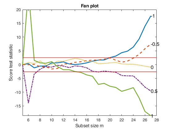
Fan plot using fidelity cards data.
Fan plot using fidelity cards data.In the example, la is the vector containing the most common values of the transformation parameter.
% Store the score test statistics for the specified values of lambda
% and automatically produce the fan plot
XX=load('loyalty.txt');
namey='Sales'
y=XX(:,end);
nameX={'Number of visits', 'Age', 'Number of persons in the family'};
X=XX(:,1:end-1);
% la = vector containing the most common values of the transformation
% parameter
la=[0 1/3 0.4 0.5];
% Store the score test statistics for the specified values of lambda
% and automatically produce the fan plot
[out]=FSRfan(y,X,'la',la,'init',size(X,2)+2,'plots',1,'lwd',3);
% The fan plot shows that even if the third root is the best value of the
% transformation parameter at the end of the search, in earlier steps it
% lies very close to the upper rejection region. The best value of the
% transformation parameter seems to be the one associated with l=0.4,
% which is always the confidence bands, but at the end of search, due to
% the presence of particular observations, it goes below the lower
% rejection line.
namey =

    'Sales'

Total estimated time to complete LMS:  0.01 seconds
Total estimated time to complete LMS:  0.02 seconds
Total estimated time to complete LMS:  0.03 seconds
Total estimated time to complete LMS:  0.02 seconds
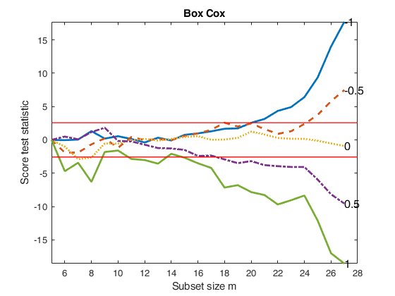
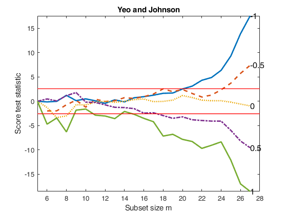
Compare BoxCox with Yeo and Johnson transformation.
Compare BoxCox with Yeo and Johnson transformation.Store values of the score test statistic for the five most common values of \lambda.
% Produce also a fan plot and display it on the screen.
% Common part to all examples: load wool dataset.
XX=load('wool.txt');
y=XX(:,end);
X=XX(:,1:end-1);
% Store the score test statistic using Box Cox transformation.
[outBC]=FSRfan(y,X,'nsamp',0);
% Store the score test statistic using Yeo and Johnson transformation.
[outYJ]=FSRfan(y,X,'family','YJ','nsamp',0);
fanplotFS(outBC,'titl','Box Cox');
fanplotFS(outYJ,'titl','Yeo and Johnson','tag','YJ');
disp('Maximum difference in absolute value')
disp(max(max(abs(outYJ.Score-outBC.Score))))
Total estimated time to complete LMS:  0.04 seconds
------------------------------
Warning: Number of subsets without full rank equal to 16.6%
Total estimated time to complete LMS:  0.04 seconds
------------------------------
Warning: Number of subsets without full rank equal to 16.6%
Total estimated time to complete LMS:  0.04 seconds
------------------------------
Warning: Number of subsets without full rank equal to 16.6%
Total estimated time to complete LMS:  0.04 seconds
------------------------------
Warning: Number of subsets without full rank equal to 16.6%
Total estimated time to complete LMS:  0.04 seconds
------------------------------
Warning: Number of subsets without full rank equal to 16.6%
Total estimated time to complete LMS:  0.04 seconds
------------------------------
Warning: Number of subsets without full rank equal to 16.6%
Total estimated time to complete LMS:  0.04 seconds
------------------------------
Warning: Number of subsets without full rank equal to 16.6%
Total estimated time to complete LMS:  0.04 seconds
------------------------------
Warning: Number of subsets without full rank equal to 16.6%
Total estimated time to complete LMS:  0.04 seconds
------------------------------
Warning: Number of subsets without full rank equal to 16.6%
Total estimated time to complete LMS:  0.04 seconds
------------------------------
Warning: Number of subsets without full rank equal to 16.6%
Maximum difference in absolute value
    0.7564
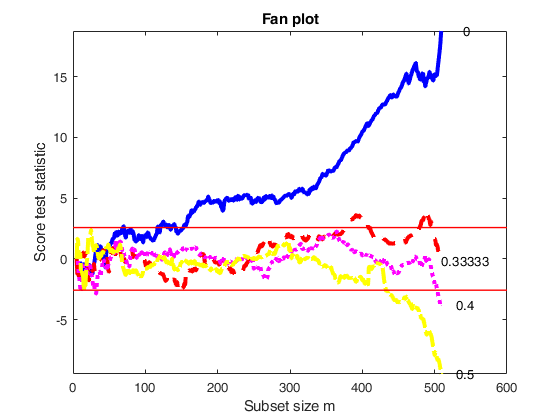
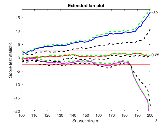
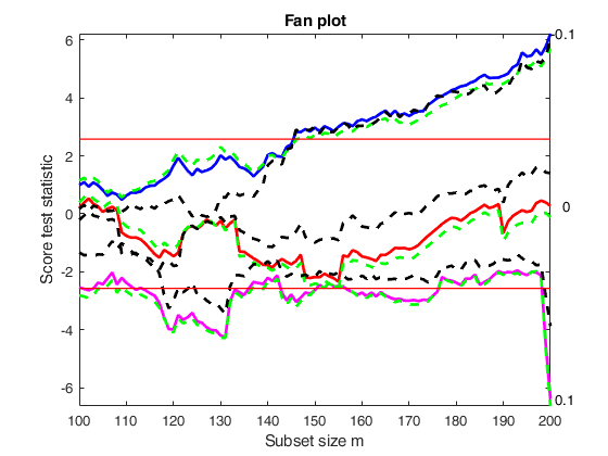
Example of monitoring of score test for positive and negative observations.
Example of monitoring of score test for positive and negative observations.
rng('default')
rng(10)
close all
n=200;
X=randn(n,3);
beta=[ 1; 1; 1];
sig=0.5;
y=X*beta+sig*randn(n,1);
disp('Fit in the true scale')
disp('R2 of the model in the true scale')
if verLessThanFS('8.1')
out=regstats(y,X,'linear',{'rsquare'});
disp(out.rsquare)
else
outlmori=fitlm(X,y);
disp(outlmori.Rsquared.Ordinary)
end
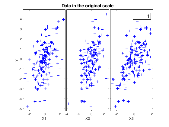
[~,~,BigAx]=yXplot(y,X,'tag','ori');
title(BigAx,'Data in the original scale')
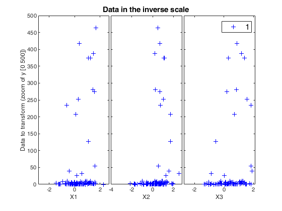
% Find the data to transform
la=-0.25;
ytra=normYJ(y,[],la,'inverse',true);
if any(isnan(ytra))
disp('response with missing values')
end
disp('Fit in the transformed scale')
disp('R2 of the model in the wrong (inverse) scale')
if verLessThanFS('8.1')
out=regstats(ytra,X,'linear',{'rsquare'});
disp(out.rsquare)
else
outlmtra=fitlm(X,ytra);
disp(outlmtra.Rsquared.Ordinary)
end
[~,~,BigAx]=yXplot(ytra,X,'tag','tra','namey','Data to transform (zoom of y [0 500])','ylimy',[0 500]);
title(BigAx,'Data in the inverse scale')
la=[ -0.5 -0.25 0];
out=FSRfan(ytra,X,'la',la,'family','YJpn','plots',1,'init',round(n/2),'msg',0);
title('Extended fan plot')
Fit in the true scale
R2 of the model in the true scale
    0.8993

Fit in the transformed scale
R2 of the model in the wrong (inverse) scale
    0.0471
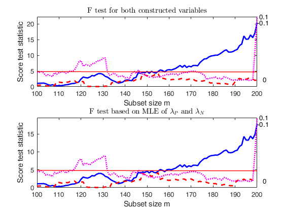
Example of monitoring all score tests (also the F test).
Example of monitoring all score tests (also the F test).
rng('default')
rng(1000)
close all
n=200;
X=randn(n,3);
beta=[ 1; 1; 1];
sig=0.5;
y=X*beta+sig*randn(n,1);
% Find the data to transform
la=0;
ytra=normYJ(y,[],la,'inverse',true);
if any(isnan(ytra))
disp('response with missing values')
end
la=[ -0.1 0 0.1];
% In this case  family is YJall
out=FSRfan(ytra,X,'la',la,'family','YJall','plots',1,'init',round(n/2),'msg',0);
Comparison of F test based on constructed variables with F test based on MLE.
Comparison of F test based on constructed variables with F test based on MLE.
rng('default')
rng(100)
close all
n=200;
X=randn(n,3);
beta=[ 1; 1; 1];
sig=0.5;
y=X*beta+sig*randn(n,1);
% Find the data to transform
la=0;
ytra=normYJ(y,[],la,'inverse',true);
if any(isnan(ytra))
disp('response with missing values')
end
la=[ -0.1 0 0.1];
% Monitor test based on MLE using option scoremle
scoremle= true;
out=FSRfan(ytra,X,'la',la,'family','YJall','plots',1,'init',round(n/2),'msg',false,'scoremle',true);
Input Arguments
Output Arguments
References
Atkinson, A.C. and Riani, M. (2000), "Robust Diagnostic Regression Analysis", Springer Verlag, New York.
Atkinson, A.C. and Riani, M. (2002a), Tests in the fan plot for robust, diagnostic transformations in regression, "Chemometrics and Intelligent Laboratory Systems", Vol. 60, pp. 87-100.
Atkinson, A.C. Riani, M., Corbellini A. (2019), The analysis of transformations for profit-and-loss data, Journal of the Royal Statistical Society, Series C, "Applied Statistics", https://doi.org/10.1111/rssc.12389
Atkinson, A.C. Riani, M. and Corbellini A. (2021), The Box–Cox Transformation: Review and Extensions, "Statistical Science", Vol. 36, pp. 239-255, https://doi.org/10.1214/20-STS778
|
|
FSRenvmdr |
FSRH |
|
|
|
Functions |
|
• The developers of the toolbox • The forward search group • Terms of Use • Acknowledgments