
|
fanBIC |
fanplot |
 |
fanBICpn
fanBICpn uses the output of FSRfan called with input option family 'YJpn' to choose la_P and la_N
Description
Examples
 Example of use of FSRfanBICpn with all default options.
Example of use of FSRfanBICpn with all default options.Load the Investment funds data.
YY=load('fondi_large.txt');
y=YY(:,2);
X=YY(:,[1 3]);
yXplot(y,X);
n=length(y);
[outFSRfan]=FSRfan(y,X,'plots',0,'init',round(n*0.3),'nsamp',10000,'la',[0 0.25 0.5 0.75 1 1.25],'msg',0,'family','YJ');
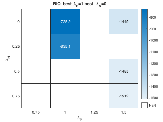
[outini]=fanBIC(outFSRfan,'plots',0);
% labest is the best value imposing the constraint that positive and
% negative observations must have the same transformation parameter.
labest=outini.labest;
% Compute test for positive and test for negative using labest
[outFSRfanpn]=FSRfan(y,X,'msg',0,'family','YJpn','la',labest,'plots',0);
% Check if two different transformations are needed for positive and negative values
out=fanBICpn(outFSRfanpn);
Analyzing la_P=0.75 and la_N=0.25
Analyzing la_P=0.75 and la_N=0
Analyzing la_P=0.75 and la_N=0.75
Analyzing la_P=0.75 and la_N=0.5
Analyzing la_P=1 and la_N=0.25
Analyzing la_P=1 and la_N=0
Analyzing la_P=1 and la_N=0.75
Analyzing la_P=1 and la_N=0.5
Analyzing la_P=1.25 and la_N=0.25
Analyzing la_P=1.25 and la_N=0
Analyzing la_P=1.25 and la_N=0.75
Analyzing la_P=1.25 and la_N=0.5
Analyzing la_P=1.5 and la_N=0.25
Analyzing la_P=1.5 and la_N=0
Analyzing la_P=1.5 and la_N=0.75
Analyzing la_P=1.5 and la_N=0.5
Example of the use of option laRangeAndStep.
Example of the use of option laRangeAndStep.Use simulated data from Atkinson Riani and Corbellini (2020)
rng('default')
rng(10)
n=1000;
p=3;
kk=200;
X=randn(n,p);
beta=[ 1; 1; 1]*0.3;
sig=0.5;
eta=X*beta;
init=6;
lapos=1.5;
laneg=0;
y=eta+sig*randn(n,1);
% Data contamination
y(1:kk)=y(1:kk)-1.9;
ypos=y>0;
ytra=y;
ytra(ypos)=normYJ(y(ypos),[],lapos,'inverse',true,'Jacobian',false);
ytra(~ypos)=normYJ(y(~ypos),[],laneg,'inverse',true,'Jacobian',false);
y=ytra;
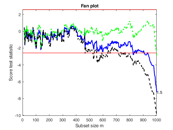
% Initial fan plot
outFSRfan=FSRfan(y,X,'la',[0.5 0.75 1 1.25 1.5],'family','YJ','plots',0,'init',init,'msg',0);
% Find best value of lambda according to BIC
% (same value of lambda for positive and negative observations).
[outUniqueLambda]=fanBIC(outFSRfan,'plots',0);
BIC=outUniqueLambda.BIC;
labest=outUniqueLambda.labest;
% Check if two different transformations are needed for positive and negative values
[outFSRfanpn]=FSRfan(y,X,'msg',0,'family','YJpn','la',labest);
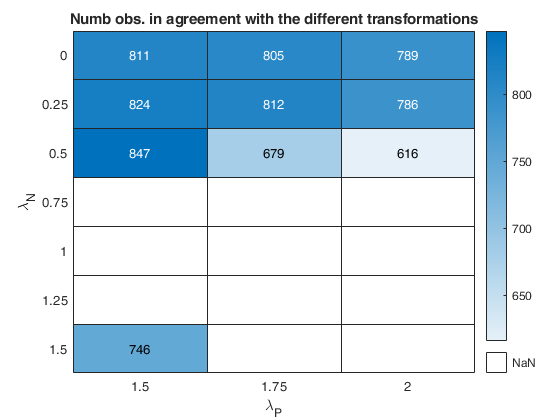
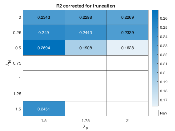
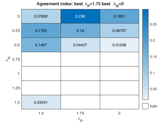
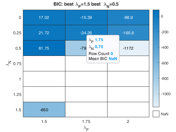
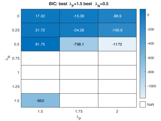
% option laRangeAndStep
laRangeAndStep=[1.5 0.25 0.5];
out=fanBICpn(outFSRfanpn,'laRangeAndStep',laRangeAndStep);
Analyzing la_P=1.5 and la_N=0.5
Analyzing la_P=1.5 and la_N=0
Analyzing la_P=1.5 and la_N=1.5
Analyzing la_P=1.5 and la_N=1
Analyzing la_P=1.5 and la_N=0.25
Analyzing la_P=1.5 and la_N=1.25
Analyzing la_P=1.5 and la_N=0.75
Analyzing la_P=1.75 and la_N=0.5
Analyzing la_P=1.75 and la_N=0
Analyzing la_P=1.75 and la_N=1.5
Analyzing la_P=1.75 and la_N=1
Analyzing la_P=1.75 and la_N=0.25
Analyzing la_P=1.75 and la_N=1.25
Analyzing la_P=1.75 and la_N=0.75
Analyzing la_P=2 and la_N=0.5
Analyzing la_P=2 and la_N=0
Analyzing la_P=2 and la_N=1.5
Analyzing la_P=2 and la_N=1
Analyzing la_P=2 and la_N=0.25
Analyzing la_P=2 and la_N=1.25
Analyzing la_P=2 and la_N=0.75

Related Examples
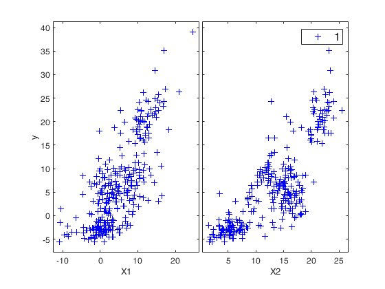
Example of the use of options fraciniFSR and plots.
Example of the use of options fraciniFSR and plots.Balance sheets data.
XX=load('BalanceSheets.txt');
% Define X and y
y=XX(:,6);
X=XX(:,1:5);
n=length(y);
la=[0 0.25 0.5 0.75 1 1.25];
[outFSRfan]=FSRfan(y,X,'plots',1,'init',round(n*0.3),'nsamp',5000,'la',la,'msg',0,'family','YJ');
[outini]=fanBIC(outFSRfan,'plots',0);
% labest is the best value imposing the constraint that positive and
% negative observations must have the same transformation parameter.
labest=outini.labest;
% Compute test for positive and test for negative using labest
indexlabest=find(labest==la);
% Find initial subset to initialize the search.
lms=outFSRfan.bs(:,indexlabest);
[outFSRfanpn]=FSRfan(y,X,'msg',0,'family','YJpn','la',labest,'plots',0,'lms',lms);
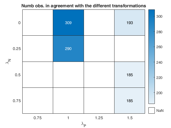
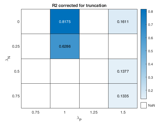
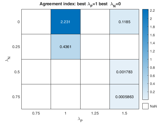
% Check if two different transformations are needed for positive and negative values
% Start monitoring the exceedances in the subset in agreement with a
% transformation from 90 per cent.
fraciniFSR=0.90;
% option plots (just show the BIC and the agreement index plot).
plots=struct;
plots.name={'BIC','AGI'};
nsamp=2000;
out=fanBICpn(outFSRfanpn,'fraciniFSR',fraciniFSR,'plots',plots,'nsamp',nsamp);
Analyzing la_P=0 and la_N=1
Analyzing la_P=0 and la_N=0.75
Analyzing la_P=0 and la_N=1.5
Analyzing la_P=0 and la_N=1.25
Analyzing la_P=0.25 and la_N=1
Analyzing la_P=0.25 and la_N=0.75
Analyzing la_P=0.25 and la_N=1.5
Analyzing la_P=0.25 and la_N=1.25
Analyzing la_P=0.5 and la_N=1
Analyzing la_P=0.5 and la_N=0.75
Analyzing la_P=0.5 and la_N=1.5
Analyzing la_P=0.5 and la_N=1.25
Analyzing la_P=0.75 and la_N=1
Analyzing la_P=0.75 and la_N=0.75
Analyzing la_P=0.75 and la_N=1.5
Analyzing la_P=0.75 and la_N=1.25
Input Arguments
Output Arguments
References
Atkinson, A.C. and Riani, M. (2000), "Robust Diagnostic Regression Analysis", Springer Verlag, New York.
Atkinson, A.C. and Riani, M. (2002a), Tests in the fan plot for robust, diagnostic transformations in regression, "Chemometrics and Intelligent Laboratory Systems", Vol. 60, pp. 87-100.
Atkinson, A.C. Riani, M., Corbellini A. (2019), The analysis of transformations for profit-and-loss data, Journal of the Royal Statistical Society, Series C, "Applied Statistics", https://doi.org/10.1111/rssc.12389
Atkinson, A.C. Riani, M. and Corbellini A. (2021), The Box–Cox Transformation: Review and Extensions, "Statistical Science", Vol. 36, pp. 239-255, https://doi.org/10.1214/20-STS778
|
|
fanBIC |
fanplot |
|
|
|
Functions |
|
• The developers of the toolbox • The forward search group • Terms of Use • Acknowledgments