fanplot
fanplot OLD FUNCTION (this function is replaced by fanplotFS and it is not updated anylonger)
Description
NOTE THAT THIS FUNCTION WILL BE REMOVED IN A FUTURE RELEASE OF FSDA BECAUSE IT IS IN CONFLICT WITH FUNCTION fanplot OF THE ECONOMETRIC TOOLBOX.
This function has been replace by function fanplotFS
fanplot with all default options.brushedUnits
=fanplot(out)
fanplot with optional arguments.brushedUnits
=fanplot(out,
Name, Value)
Examples
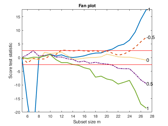
 fanplot with all default options.
fanplot with all default options.load the wool data
XX=load('wool.txt');
y=XX(:,end);
X=XX(:,1:end-1);
% FSRfan and fanplot with all default options
[out]=FSRfan(y,X);
fanplotFS(out);
Total estimated time to complete LMS:  0.12 seconds
------------------------------
Warning: Number of subsets without full rank equal to 17.1%
Total estimated time to complete LMS:  0.02 seconds
------------------------------
Warning: Number of subsets without full rank equal to 17.1%
Total estimated time to complete LMS:  0.02 seconds
------------------------------
Warning: Number of subsets without full rank equal to 17.1%
Total estimated time to complete LMS:  0.02 seconds
------------------------------
Warning: Number of subsets without full rank equal to 17.1%
Total estimated time to complete LMS:  0.02 seconds
------------------------------
Warning: Number of subsets without full rank equal to 17.1%
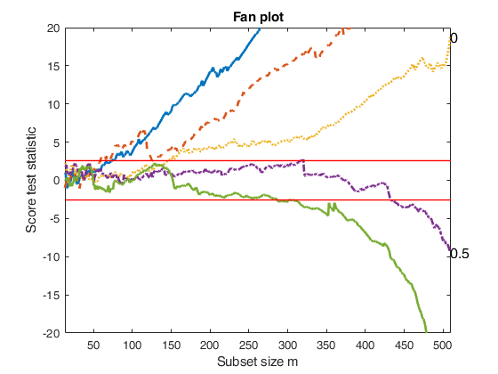
fanplot with optional arguments.
fanplot with optional arguments.FSRfan and fanplot with specified lambda
load('loyalty.txt');
y=loyalty(:,4);
X=loyalty(:,1:3);
% la = vector contanining the most common values of the transformation
% parameter
la=[-1 -0.5 0 0.5 1];
[out]=FSRfan(y,X,'la',la);
fanplotFS(out);
Total estimated time to complete LMS:  0.02 seconds
Total estimated time to complete LMS:  0.03 seconds
Total estimated time to complete LMS:  0.01 seconds
Total estimated time to complete LMS:  0.02 seconds
Total estimated time to complete LMS:  0.02 seconds
Related Examples
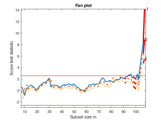
fanplot with option highlight (second example).
fanplot with option highlight (second example).
load gasoline.mat
y=gasoline{:,2};
X=gasoline{:,1};
[out]=FSRfan(y,X,'la', [-1 0 1]);
% In the code below, option highlight enables us to understand when units
% [21 18 33 77] join the subset for the difference values of lambda
fanplotFS(out,'highlight',[ 21 18 33 77]);
Total estimated time to complete LMS:  0.00 seconds
Total estimated time to complete LMS:  0.00 seconds
Total estimated time to complete LMS:  0.00 seconds
Steps of entry of selected units when la= -1
    95    21
    99    18
   100    33
   107    77

Steps of entry of selected units when la= 0
    92    21
    99    18
   100    33
   107    77

Steps of entry of selected units when la= 1
    92    21
    99    18
   100    33
   107    77
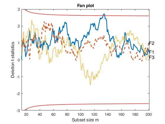
fanplot based on the output of FSRaddt.
fanplot based on the output of FSRaddt.
n=200;
p=3;
randn('state', 123456);
X=randn(n,p);
% Uncontaminated data
y=randn(n,1);
nameX={'F1','F2','F3'};
[out]=FSRaddt(y,X,'plots',0);
% out.la contains the names of the variables which have to be shown
out.la=nameX;
fanplotFS(out);
Total estimated time to complete LMS:  0.01 seconds
Total estimated time to complete LMS:  0.01 seconds
Total estimated time to complete LMS:  0.01 seconds
Input Arguments
Output Arguments
References
Atkinson, A.C. and Riani, M. (2000), "Robust Diagnostic Regression Analysis", Springer Verlag, New York.
Atkinson, A.C. and Riani, M. (2002a), Tests in the fan plot for robust, diagnostic transformations in regression, "Chemometrics and Intelligent Laboratory Systems", Vol. 60, pp. 87-100.
Atkinson, A.C. Riani, M., Corbellini A. (2019), The analysis of transformations for profit-and-loss data, Journal of the Royal Statistical Society, Series C, "Applied Statistics", https://doi.org/10.1111/rssc.12389
Atkinson, A.C. Riani, M. and Corbellini A. (2021), The Box–Cox Transformation: Review and Extensions, "Statistical Science", Vol. 36, pp. 239-255, https://doi.org/10.1214/20-STS778