LXS

LXS computes the Least Median of Squares (LMS) or Least Trimmed Squares (LTS) estimators

Syntax

Description

example

out =LXS(y, X) LXS with default input and output.

example

out =LXS(y, X, Name, Value) LXS with optional arguments.

example

[out , varargout] =LXS(___) LXS with optional output.

Examples

expand all

  • LXS with default input and output.
  • Compute LMS estimator without reweighting, add intercept to matrix X and do not produce plots.

    n=200;
    p=3;
    randn('state', 123456);
    X=randn(n,p);
    y=randn(n,1);
    y(1:5)=y(1:5)+6;
    [out]=LXS(y,X);

  • LXS with optional arguments.
  • Compute LMS estimator, reweight and plot the residuals.

    n=200;
    p=3;
    randn('state', 123456);
    X=randn(n,p);
    y=randn(n,1);
    y(1:5)=y(1:5)+6;
    [out]=LXS(y,X,'rew',1,'plots',1);

  • LXS with optional output.
  • Generating the C matrix containing the indices of the subsamples extracted for computing the estimate (the so called elemental sets).

    n=200;
    p=3;
    randn('state', 123456);
    X=randn(n,p);
    y=randn(n,1);
    y(1:5)=y(1:5)+6;
    [out,C]=LXS(y,X);

    Related Examples

    expand all

  • Reweighted LTS estimator.
  • Compute reweighted LTS estimator and produce the plot of residuals.

    n=200;
    p=3;
    randn('state', 123456);
    X=randn(n,p);
    y=randn(n,1);
    y(1:5)=y(1:5)+6;
    [out]=LXS(y,X,'rew',1,'lms',0,'plots',1);

  • Specifying the number of subsamples.
  • Compute LMS estimator, without plots using 20000 subsamples.

    n=200;
    p=3;
    randn('state', 123456);
    X=randn(n,p);
    y=randn(n,1);
    y(1:5)=y(1:5)+6;
    [out]=LXS(y,X,'nsamp',20000);

  • Specifying a confidence level.
  • Compute reweighted LMS and use a confidence level for outlier detection equal to 0.999.

    n=200;
    p=3;
    randn('state', 123456);
    X=randn(n,p);
    y=randn(n,1);
    y(1:5)=y(1:5)+6;
    [out]=LXS(y,X,'rew',1,'conflev',0.999);

  • Using fast options.
  • Compute LTS using fast options detection equal to 0.999.

    lms=struct;
    % Do 5 refining steps for each elemental subset
    lms.refsteps=5;
    % Store the best 10 subsets
    lms.bestr=10;
    n=200;
    p=3;
    randn('state', 123456);
    X=randn(n,p);
    y=randn(n,1);
    y(1:5)=y(1:5)+6;
    [out]=LXS(y,X,'lms',lms,'plots',1);

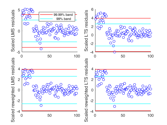
  • We compare the output of different procedures: only the reweighted LTS seems to detect half of the outlier with a Bonferroni significance level.
  • close all;
    state=100;
    randn('state', state);
    n=100;
    X=randn(n,3);
    bet=[3;4;5];
    y=3*randn(n,1)+X*bet;
    y(1:20)=y(1:20)+13;
    % Define nominal confidence level
    conflev=[0.99,1-0.01/length(y)];
    % Define number of subsets
    nsamp=3000;
    % Define the main title of the plots
    titl='';
    % LMS with no reweighting
    [outLMS]=LXS(y,X,'nsamp',nsamp,'conflev',conflev(1));
    h=subplot(2,2,1)
    laby='Scaled LMS residuals';
    resindexplot(outLMS.residuals,'h',h,'title',titl,'laby',laby,'numlab','','conflev',conflev)
    % LTS with no reweighting
    h=subplot(2,2,2);
    [outLTS]=LXS(y,X,'nsamp',nsamp,'conflev',conflev(1),'lms',0);
    laby='Scaled LTS residuals';
    resindexplot(outLTS.residuals,'h',h,'title',titl,'laby',laby,'numlab','','conflev',conflev);
    % LMS with reweighting
    [outLMSr]=LXS(y,X,'nsamp',nsamp,'conflev',conflev(1),'rew',1);
    h=subplot(2,2,3);
    laby='Scaled reweighted LMS residuals';
    resindexplot(outLMSr.residuals,'h',h,'title',titl,'laby',laby,'numlab','','conflev',conflev)
    % LTS with reweighting
    [outLTSr]=LXS(y,X,'nsamp',nsamp,'conflev',conflev(1),'rew',1,'lms',0);
    h=subplot(2,2,4);
    laby='Scaled reweighted LTS residuals';
    resindexplot(outLTSr.residuals,'h',h,'title',titl,'laby',laby,'numlab','','conflev',conflev);
    % By simply changing the seed to 543 (state=543), using a Bonferroni size of 1%, no unit is declared as outlier.
    Warning: Using 'state' to set RANDN's internal state causes RAND, RANDI, and
    RANDN to use legacy random number generators.  This syntax is not recommended.
    See <a href="matlab:helpview([docroot '\techdoc\math\math.map'],'update_random_number_generator')">Replace Discouraged Syntaxes of rand and randn</a> to use RNG to replace the
    old syntax. 
    Total estimated time to complete LMS:  0.01 seconds 
    
    h = 
    
      Axes with properties:
    
                 XLim: [0 1]
                 YLim: [0 1]
               XScale: 'linear'
               YScale: 'linear'
        GridLineStyle: '-'
             Position: [0.1300 0.5838 0.3347 0.3412]
                Units: 'normalized'
    
      Use GET to show all properties
    
    Total estimated time to complete LTS:  0.01 seconds 
    Total estimated time to complete LMS:  0.01 seconds 
    Total estimated time to complete LTS:  0.01 seconds 
    
    Click here for the graphical output of this example (link to Ro.S.A. website)

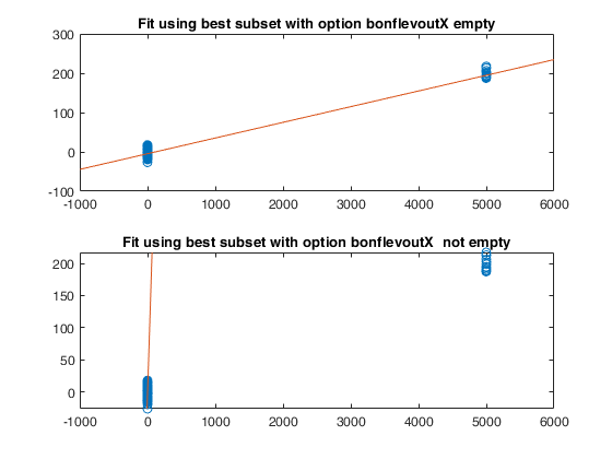
  • Example of the use of option bonflevoutX.
  • In this example a set of remote units is added to a cloud of points.

    % The purpose of this example is to show that while best LMS using all
    % default options contains some of the remote units. In order to make sure
    % that the remote units are excluded from the best LMS subset it is
    % necessary to use option bonflevoutX.
    rng('default')
    rng(10000)
    n=100;
    p=1;
    X=randn(n,p);
    epsil=10;
    beta=ones(p,1);
    y=X*beta+randn(n,1)*epsil;
    % Add 10 very remote points
    add=10;
    Xadd=X(1:add,:)+5000;
    yadd=y(1:add)+200;
    Xall=[X;Xadd];
    yall=[y;yadd];
    out=LXS(yall,Xall);
    subplot(2,1,1)
    plot(Xall,yall,'o')
    xylim=axis;
    line(xylim(1:2),out.beta(1)+out.beta(2)*xylim(1:2))
    title('Fit using best subset with option bonflevoutX empty')
    subplot(2,1,2)
    plot(Xall,yall,'o')
    out=LXS(yall,Xall,'bonflevoutX',0.99);
    line(xylim(1:2),out.beta(1)+out.beta(2)*xylim(1:2))
    ylim(xylim(3:4));
    title('Fit using best subset with option bonflevoutX  not empty')
    Total estimated time to complete LMS:  0.01 seconds 
    Total estimated time to complete LMS:  0.05 seconds 
    ------------------------------
    Warning: Number of subsets without full rank or excluded because containing remote units in the X space equal to 17.1 %
    
    Click here for the graphical output of this example (link to Ro.S.A. website)

  • LXS with optional arguments.
  • Compute LTS estimator, reweight and plot the residuals.

    % Use a confidence level for reweighting using 0.99 and a simultaneous
    % confidence interval for outlier detection
    n=200;
    p=3;
    randn('state', 123456);
    X=randn(n,p);
    y=randn(n,1);
    y(1:5)=y(1:5)+6;
    [out]=LXS(y,X,'rew',1,'conflev',1-0.01/n,'conflevrew',0.99,'plots',1);

    Input Arguments

    expand all

    y — Response variable. Vector.

    A vector with n elements that contains the response variable. It can be either a row or a column vector.

    Data Types: single| double

    X — Predictor variables. Matrix.

    Data matrix of explanatory variables (also called 'regressors') of dimension (n x p-1). Rows of X represent observations, and columns represent variables.

    Missing values (NaN's) and infinite values (Inf's) are allowed, since observations (rows) with missing or infinite values will automatically be excluded from the computations.

    Data Types: single| double

    Name-Value Pair Arguments

    Specify optional comma-separated pairs of Name,Value arguments. Name is the argument name and Value is the corresponding value. Name must appear inside single quotes (' '). You can specify several name and value pair arguments in any order as Name1,Value1,...,NameN,ValueN.

    Example: 'bdp',0.4 , 'bonflevoutX',0.95 , 'conflev',0.99 , 'conflevrew',0.99 , 'h',round(n*0,75) , 'intercept',false , 'lms',1 , 'nocheck',true , 'nomes',true , 'msg',false , 'nsamp',0 , 'rew',true , 'SmallSampleCor',3 , 'yxsave',1 , 'plots',1

    bdp —breakdown point.scalar.

    It measures the fraction of outliers the algorithm should resist. In this case any value greater than 0 but smaller or equal than 0.5 will do fine. If on the other hand the purpose is subgroups detection then bdp can be greater than 0.5. In any case however n*(1-bdp) must be greater than p. If this condition is not fulfilled an error will be given. Please specify h or bdp not both.

    Example: 'bdp',0.4

    Data Types: double

    bonflevoutX —remote units in the X space.scalar | empty (default).

    If the design matrix X contains several high leverage units (that is units which are very far from the bulk of the data), it may happen that the best subset may include some of these units.

    If boflevoutX is not empty, outlier detection procedure FSM is applied to the design matrix X, using name/pair option 'bonflev',bonflevoutX. The extracted subsets which contain at least one unit declared as outlier in the X space by FSM are removed (more precisely they are treated as singular subsets) from the list of candidate subsets to find the LXS solution. The default value of bonflevoutX is empty, that is FSM is not invoked.

    Example: 'bonflevoutX',0.95

    Data Types: double

    conflev —Confidence level which is used to declare units as outliers.scalar Usually conflev=0.

    95, 0.975 0.99 (individual alpha) or 1-0.05/n, 1-0.025/n, 1-0.01/n (simultaneous alpha).

    Default value is 0.975

    Example: 'conflev',0.99

    Data Types: double

    conflevrew —Confidence level for use for reweighting.scalar.

    Number between 0 and 1 containing confidence level which is used to do the reweighting step. Default value is the one specified in previous option conflev.

    Example: 'conflevrew',0.99

    Data Types: double

    h —The number of observations that have determined the least trimmed squares estimator.scalar.

    The number of observations that have determined the least trimmed squares estimator. h is an integer greater than p (number of columns of matrix X including the intercept but smaller then n. If the purpose is outlier detection than h does not have to be smaller than [0.5*(n+p+1)] (default value). On the other hand if the purpose is to find subgroups of homogeneous observations h can be smaller than [0.5*(n+p+1)]. If h <p+1 an error will be given.

    Example: 'h',round(n*0,75)

    Data Types: double

    intercept —Indicator for constant term.true (default) | false.

    Indicator for the constant term (intercept) in the fit, specified as the comma-separated pair consisting of 'Intercept' and either true to include or false to remove the constant term from the model.

    Example: 'intercept',false

    Data Types: boolean

    lms —Estimation method.scalar, vector | structure.

    If lms is a scalar = 1 (default) Least Median of Squares is computed, else if lms is a scalar = 2 fast lts with the all default options is used else if lms is a scalar different from 1 and 2 standard lts is used (without concentration steps) else if lms is a struct fast lts (with concentration steps) is used.

    In this case the user can control the following options: lms.refsteps : scalar defining number of refining iterations in each subsample (default = 3). refsteps = 0 means "raw-subsampling" without iterations.

    lms.reftol : scalar. Default value of tolerance for the refining steps The default value is 1e-6.

    lms.bestr : scalar defining number of "best betas" to remember from the subsamples. These will be later iterated until convergence (default=5).

    lms.refstepsbestr : scalar defining number of refining iterations for each best subset (default = 50).

    lms.reftolbestr : scalar. Default value of tolerance for the refining steps for each of the best subsets The default value is 1e-8.

    Example: 'lms',1

    Data Types: double

    nocheck —Check input arguments.boolean.

    If nocheck is equal to true no check is performed on matrix y and matrix X. Notice that when no check is true y and X are left unchanged, that is the additional column of ones for the intercept is not added. As default nocheck=false. The controls on h, bdp and nsamp still remain.

    Example: 'nocheck',true

    Data Types: boolean

    nomes —It controls whether to display or not on the screen messages about estimated time to compute LMS (LTS) .boolean.

    If nomes is equal to true no message about estimated time to compute LMS (LTS) is displayed, else if nomes is equal to false (default), a message about estimated time is displayed.

    Example: 'nomes',true

    Data Types: logical

    msg —It controls whether to display or not messages on the screen.boolean.

    If msg==true (default) messages are displayed on the screen about estimated time to compute the estimator and the warnings about 'MATLAB:rankDeficientMatrix', 'MATLAB:singularMatrix' and 'MATLAB:nearlySingularMatrix' are set to off else no message is displayed on the screen

    Example: 'msg',false

    Data Types: logical

    nsamp —Number of subsamples which will be extracted to find the robust estimator or matrix with preextracted subsamples.scalar | matrix.

    If nsamp=0 all subsets will be extracted. They will be (n choose p). If nsamp is (say) 200, 200 subsets will be extracted. If nsamp is a matrix of size r-by-p, it contains in the rows the subsets which sill have to be extracted.

    For example, if p=3 and nsamp=[ 2 4 9; 23 45 49; 90 34 1];

    the first subset is made up of units [2 4 9], the second subset of units [23 45 49] and the third subset of units [90 34 1];

    Remark: if the number of all possible subset is <1000 the default is to extract all subsets, otherwise just 1000 if fastLTS is used (lms=2 or lms is a structure) or 3000 for standard LTS or LMS.

    Example: 'nsamp',0

    Data Types: double

    rew —LXS reweighted.boolean.

    If rew=true the reweighted version of LTS (LMS) is used and the output quantities refer to the reweighted version else no reweighting is performed (default).

    Example: 'rew',true

    Data Types: logical

    SmallSampleCor —Small sample correction factor to control empirical size of the test.scalar equal to 0 (default) | 1 | 2 | 3 | 4.

    - If SmallSampleCor=0 (default) no small sample correction;

    - If SmallSampleCor=1 in the reweighting step the nominal threshold based on $\chi^2_{0.99}$ is multiplied by the small sample correction factor which guarrantees that the empirical size of the test is equal to the nominal size;

    - If SmallSampleCor =2 Gervini and Yohai procedure is called with 'iterating' false and 'alpha' 0.99 is invoked, that is: weights=GYfilt(stdres,'iterating',false,'alpha',0.99);

    - If SmallSampleCor =3 Gervini and Yohai procedure called with 'iterating' true and 'alpha' 0.99 is invoked, that is: weights=GYfilt(stdres,'iterating',true,'alpha',0.99);

    - If SmallSampleCor =4 $\chi^2_{0.99}$ threshold is used that is: weights = abs(stdres)<=sqrt(chi2inv(0.99,1));

    Example: 'SmallSampleCor',3

    Data Types: double

    yxsave —the response vector y and data matrix X are saved into the output structure out.scalar.

    Default is 0, i.e. no saving is done.

    Example: 'yxsave',1

    Data Types: double

    plots —Plot on the screen.scalar | structure.

    If plots = 1, a plot which shows the robust residuals against index number is shown on the screen. The confidence level which is used to draw the horizontal lines associated with the bands for the residuals is as specified in input option conflev. If conflev is missing a nominal 0.975 confidence interval will be used.

    Example: 'plots',1

    Data Types: double

    Output Arguments

    expand all

    out — description Structure

    A structure containing the following fields

    Value Description
    rew

    boolean. if out.rew=true all subsequent output refers to reweighted else no reweighting is done.

    beta

    Vector of beta LTS (LMS) coefficient estimates, including the intercept when options.intercept=true.

    out.beta=[intercept slopes].

    bs

    p x 1 vector containing the units forming subset associated with bLMS (bLTS).

    residuals

    Vector containing the standardized residuals from the regression.

    scale

    Scale estimate of the residuals.

    weights

    Vector like y containing weights. The elements of this vector are 0 or 1.

    These weights identify the h observations which are used to compute the final LTS (LMS) estimate.

    sum(out.weights)=h if there is not a perfect fit otherwise sum(out.weights) can be greater than h

    h

    The number of observations that have determined the LTS (LMS) estimator, i.e. the value of h.

    outliers

    row vector containing the list of the units declared as outliers using confidence level specified in input scalar conflev.

    conflev

    confidence level which is used to declare outliers.

    Remark: scalar out.conflev will be used to draw the horizontal lines (confidence bands) in the plots

    singsub

    Number of subsets wihtout full rank. Notice that if this number is greater than 0.1*(number of subsamples) a warning is produced on the screen

    class

    'LTS' or 'LMS'.

    y

    response vector Y. The field is present only if option yxsave is set to 1.

    X

    data matrix X. The field is present only if option yxsave is set to 1.

    varargout —C : Indexes of the extracted subsamples. Matrix

    Matrix containing the indexes of the subsamples extracted for computing the estimate (the so called elemental sets). For example, if C(3,:)=[2 5 20], implies that the third extracted subsample is formed by units 2, 5 and 20.

    References

    Rousseeuw P.J., Leroy A.M. (1987), "Robust regression and outlier detection", Wiley.

    See Also

    | | |

    This page has been automatically generated by our routine publishFS