LTSts

LTSts extends LTS estimator to time series

Syntax

out=LTSts(y)example
out=LTSts(y,Name,Value)example
[out, varargout]=LTSts(___)example

Description

It is possible to set a model with a trend (up to third order), a seasonality (constant or of varying amplitude and with a different number of harmonics) and a level shift (in this last case it is possible to specify the window in which level shift has to be searched for).

example

out =LTSts(y) Simulated data with linear trend and level shift.

example

out =LTSts(y, Name, Value) Airline data: linear trend + just one harmonic for seasonal component.

example

[out, varargout] =LTSts(___) Model with linear trend and six harmonics for seasonal component.

Examples

expand all

Simulated data with linear trend and level shift.

No seasonal component.

rng('default')
T=45;
a=1;
b=0.8;
sig=1;
seq=(1:T)';
y=a+b*seq+sig*randn(T,1);
% Add a level shift in the simulated series
y(round(T/2):end)=y(round(T/2):end)+10;
% model with a linear trend, non seasonal and level shift
model=struct;
model.trend=1;
model.seasonal=0;
% Potential level shift position is investigated in positions:
% t=11, t=12, ..., t=T-10.
model.lshift=11:T-10;
out=LTSts(y,'model',model,'plots',1);
% Using the notation of the paper RPRH: A=1, B=1, G=0 and $\delta_1>0$.
str=strcat('A=1, B=0, G=0, $\delta_2=',num2str(out.posLS),'$');
title(findobj(gcf,'-regexp','Tag','LTSts:ts'),str,'interpreter','latex');

Airline data: linear trend + just one harmonic for seasonal component.

Load airline data.

%   1949 1950 1951 1952 1953 1954 1955 1956 1957 1958 1959 1960
y = [112  115  145  171  196  204  242  284  315  340  360  417    % Jan
118  126  150  180  196  188  233  277  301  318  342  391    % Feb
132  141  178  193  236  235  267  317  356  362  406  419    % Mar
129  135  163  181  235  227  269  313  348  348  396  461    % Apr
121  125  172  183  229  234  270  318  355  363  420  472    % May
135  149  178  218  243  264  315  374  422  435  472  535    % Jun
148  170  199  230  264  302  364  413  465  491  548  622    % Jul
148  170  199  242  272  293  347  405  467  505  559  606    % Aug
136  158  184  209  237  259  312  355  404  404  463  508    % Sep
119  133  162  191  211  229  274  306  347  359  407  461    % Oct
104  114  146  172  180  203  237  271  305  310  362  390    % Nov
118  140  166  194  201  229  278  306  336  337  405  432 ]; % Dec
y=(y(:));
yr = repmat((1949:1960),12,1);
mo = repmat((1:12)',1,12);
time = datestr(datenum(yr(:),mo(:),1));
ts = timeseries(y(:),time,'name','AirlinePassengers');
ts.TimeInfo.Format = 'dd-mmm-yyyy';
tscol = tscollection(ts);
% plot airline data
plot(ts)
% linear trend + just one harmonic for seasonal component
model=struct;
model.trend=1;              % linear trend
model.s=12;                 % monthly time series
model.seasonal=1;           % just one harmonic
model.lshift=0;             % no level shift
out=LTSts(y,'model',model,'dispresults',true);
close all
% Plot real and fitted values
plot(y,'Linewidth',1.5);
hold('on')
plot(out.yhat,'r--','Linewidth',1.5)
legend({'Real values','Fitted values'},'Location','SouthEast','interpreter','LaTeX','FontSize',14)
numpar = {'model parameters:' , 'A=1, B=1, G=0, $\delta_1=0$'};
title(gca,numpar,'interpreter','LaTeX','FontSize',16);

Model with linear trend and six harmonics for seasonal component.

Load airline data.

%   1949 1950 1951 1952 1953 1954 1955 1956 1957 1958 1959 1960
y = [112  115  145  171  196  204  242  284  315  340  360  417    % Jan
118  126  150  180  196  188  233  277  301  318  342  391    % Feb
132  141  178  193  236  235  267  317  356  362  406  419    % Mar
129  135  163  181  235  227  269  313  348  348  396  461    % Apr
121  125  172  183  229  234  270  318  355  363  420  472    % May
135  149  178  218  243  264  315  374  422  435  472  535    % Jun
148  170  199  230  264  302  364  413  465  491  548  622    % Jul
148  170  199  242  272  293  347  405  467  505  559  606    % Aug
136  158  184  209  237  259  312  355  404  404  463  508    % Sep
119  133  162  191  211  229  274  306  347  359  407  461    % Oct
104  114  146  172  180  203  237  271  305  310  362  390    % Nov
118  140  166  194  201  229  278  306  336  337  405  432 ]; % Dec
y=(y(:));
model=struct;
model.trend=1;              % linear trend
model.s=12;                 % monthly time series
model.seasonal=6;           % six harmonics
model.lshift=0;             % no level shift
out=LTSts(y,'model',model);
close all
% Plot real and fitted values
plot(y,'Linewidth',1.5);
hold('on')
plot(out.yhat,'r--','Linewidth',1.5)
legend({'Real values','Fitted values'},'Location','SouthEast','interpreter','LaTeX','FontSize',14)
numpar = {'model parameters:' , 'A=1, B=6, G=0, $\delta_1=0$'};
title(gca,numpar,'interpreter','LaTeX','FontSize',16);

Related Examples

expand all

Model with linear trend, two harmonics for seasonal component and varying amplitude using a linear trend (1).

% Load airline data.
%   1949 1950 1951 1952 1953 1954 1955 1956 1957 1958 1959 1960
y = [112  115  145  171  196  204  242  284  315  340  360  417    % Jan
118  126  150  180  196  188  233  277  301  318  342  391    % Feb
132  141  178  193  236  235  267  317  356  362  406  419    % Mar
129  135  163  181  235  227  269  313  348  348  396  461    % Apr
121  125  172  183  229  234  270  318  355  363  420  472    % May
135  149  178  218  243  264  315  374  422  435  472  535    % Jun
148  170  199  230  264  302  364  413  465  491  548  622    % Jul
148  170  199  242  272  293  347  405  467  505  559  606    % Aug
136  158  184  209  237  259  312  355  404  404  463  508    % Sep
119  133  162  191  211  229  274  306  347  359  407  461    % Oct
104  114  146  172  180  203  237  271  305  310  362  390    % Nov
118  140  166  194  201  229  278  306  336  337  405  432 ]; % Dec
y=(y(:));
model=struct;
model.trend=1;              % linear trend
model.s=12;                 % monthly time series
model.seasonal=102;         % two harmonics with time varying seasonality
model.lshift=0;             % no level shift
out=LTSts(y,'model',model);
close all
% Plot real and fitted values
plot(y,'Linewidth',1.5);
hold('on')
plot(out.yhat,'r--','Linewidth',1.5)
legend({'Real values','Fitted values'},'Location','SouthEast','interpreter','LaTeX','FontSize',14)
numpar = {'model parameters:' , 'A=1, B=2, G=1, $\delta_1=0$'};
title(gca,numpar,'interpreter','LaTeX','FontSize',16);

Model with linear trend, six harmonics for seasonal component and varying amplitude using a linear trend (2).

% Load airline data.
%   1949 1950 1951 1952 1953 1954 1955 1956 1957 1958 1959 1960
y = [112  115  145  171  196  204  242  284  315  340  360  417    % Jan
118  126  150  180  196  188  233  277  301  318  342  391    % Feb
132  141  178  193  236  235  267  317  356  362  406  419    % Mar
129  135  163  181  235  227  269  313  348  348  396  461    % Apr
121  125  172  183  229  234  270  318  355  363  420  472    % May
135  149  178  218  243  264  315  374  422  435  472  535    % Jun
148  170  199  230  264  302  364  413  465  491  548  622    % Jul
148  170  199  242  272  293  347  405  467  505  559  606    % Aug
136  158  184  209  237  259  312  355  404  404  463  508    % Sep
119  133  162  191  211  229  274  306  347  359  407  461    % Oct
104  114  146  172  180  203  237  271  305  310  362  390    % Nov
118  140  166  194  201  229  278  306  336  337  405  432 ]; % Dec
y=(y(:));
model=struct;
model.trend=1;              % linear trend
model.s=12;                 % monthly time series
model.seasonal=106;         % six harmonics with linear time varying seasonality
model.lshift=0;             % no level shift
% out=fitTSLS(y,'model',model);
out=LTSts(y,'model',model);
close all
% Plot real and fitted values
plot(y,'Linewidth',1.5);
hold('on')
plot(out.yhat,'r--','Linewidth',1.5)
legend({'Real values','Fitted values'},'Location','SouthEast','interpreter','LaTeX','FontSize',14)
numpar = {'model parameters:' , 'A=1, B=6, G=1, $\delta_1=0$'};
title(gca,numpar,'interpreter','LaTeX','FontSize',16);

Contaminated time series with upward level shift.

Model with linear trend, six harmonics for seasonal component and varying amplitude using a linear trend).

% Load airline data.
%   1949 1950 1951 1952 1953 1954 1955 1956 1957 1958 1959 1960
y = [112  115  145  171  196  204  242  284  315  340  360  417    % Jan
118  126  150  180  196  188  233  277  301  318  342  391    % Feb
132  141  178  193  236  235  267  317  356  362  406  419    % Mar
129  135  163  181  235  227  269  313  348  348  396  461    % Apr
121  125  172  183  229  234  270  318  355  363  420  472    % May
135  149  178  218  243  264  315  374  422  435  472  535    % Jun
148  170  199  230  264  302  364  413  465  491  548  622    % Jul
148  170  199  242  272  293  347  405  467  505  559  606    % Aug
136  158  184  209  237  259  312  355  404  404  463  508    % Sep
119  133  162  191  211  229  274  306  347  359  407  461    % Oct
104  114  146  172  180  203  237  271  305  310  362  390    % Nov
118  140  166  194  201  229  278  306  336  337  405  432 ]; % Dec
y=(y(:));
yLS=y;
yLS(55:end)=yLS(55:end)+130;
model=struct;
model.trend=1;                          % linear trend
model.s=12;                             % monthly time series
model.seasonal=1;
model.lshift=14:length(yLS)-13;         % impose level shift
out=LTSts(yLS,'model',model);
close all
% Plot real and fitted values
plot(yLS,'Linewidth',1.5);
hold('on')
plot(out.yhat,'r--','Linewidth',1.5)
legend({'Real values','Fitted values'},'Location','SouthEast','interpreter','LaTeX','FontSize',14)
% Using the notation of the paper RPRH: A=1, B=1, G=0 and $\delta_1>0$.
str=strcat('A=1, B=1, G=0, $\delta_2=',num2str(out.posLS),'$');
numpar = {'model parameters:' , str};
title(gca,numpar,'interpreter','LaTeX','FontSize',16);

Contaminated time series with downward level shift.

Model with linear trend, three harmonics for seasonal component and varying amplitude using a linear trend).

% Load airline data.
%   1949 1950 1951 1952 1953 1954 1955 1956 1957 1958 1959 1960
y = [112  115  145  171  196  204  242  284  315  340  360  417    % Jan
118  126  150  180  196  188  233  277  301  318  342  391    % Feb
132  141  178  193  236  235  267  317  356  362  406  419    % Mar
129  135  163  181  235  227  269  313  348  348  396  461    % Apr
121  125  172  183  229  234  270  318  355  363  420  472    % May
135  149  178  218  243  264  315  374  422  435  472  535    % Jun
148  170  199  230  264  302  364  413  465  491  548  622    % Jul
148  170  199  242  272  293  347  405  467  505  559  606    % Aug
136  158  184  209  237  259  312  355  404  404  463  508    % Sep
119  133  162  191  211  229  274  306  347  359  407  461    % Oct
104  114  146  172  180  203  237  271  305  310  362  390    % Nov
118  140  166  194  201  229  278  306  336  337  405  432 ]; % Dec
y=(y(:));
yLS=y;
yLS(35:end)=yLS(35:end)-300;
model=struct;
model.trend=1;              % linear trend
model.s=12;                 % monthly time series
model.seasonal=103;
model.lshift=26:length(yLS)-25;
out=LTSts(yLS,'model',model,'msg',0);
close all
% Plot real and fitted values
plot(yLS,'Linewidth',1.5);
hold('on')
plot(out.yhat,'r--','Linewidth',1.5)
legend({'Real values','Fitted values'},'Location','SouthEast','interpreter','LaTeX','FontSize',14)
% Using the notation of the paper RPRH: A=1, B=3, G=1 and $\delta_1>0$.
str=strcat('A=1, B=3, G=1, $\delta_2=',num2str(out.posLS),'$');
numpar = {'model parameters:' , str};
title(gca,numpar,'interpreter','LaTeX','FontSize',16);

Model with an explanatory variable using log-transformed series.

Load airline data.

%   1949 1950 1951 1952 1953 1954 1955 1956 1957 1958 1959 1960
y = [112  115  145  171  196  204  242  284  315  340  360  417    % Jan
118  126  150  180  196  188  233  277  301  318  342  391    % Feb
132  141  178  193  236  235  267  317  356  362  406  419    % Mar
129  135  163  181  235  227  269  313  348  348  396  461    % Apr
121  125  172  183  229  234  270  318  355  363  420  472    % May
135  149  178  218  243  264  315  374  422  435  472  535    % Jun
148  170  199  230  264  302  364  413  465  491  548  622    % Jul
148  170  199  242  272  293  347  405  467  505  559  606    % Aug
136  158  184  209  237  259  312  355  404  404  463  508    % Sep
119  133  162  191  211  229  274  306  347  359  407  461    % Oct
104  114  146  172  180  203  237  271  305  310  362  390    % Nov
118  140  166  194  201  229  278  306  336  337  405  432 ]; % Dec
y=(y(:));
y1=log(y);
% Model with linear trend, two harmonics for seasonal component and
% varying amplitude using a linear trend).
model=struct;
model.trend=1;              % linear trend
model.s=12;                 % monthly time series
model.seasonal=106;
model.lshift=0;
model.X=randn(length(y),1);
out=LTSts(y1,'model',model);
close all
% Plot real and fitted values
plot(y1,'Linewidth',1.5);
hold('on')
plot(out.yhat,'r--','Linewidth',1.5)
legend({'Real values','Fitted values'},'Location','SouthEast','interpreter','LaTeX','FontSize',14)
% Using the notation of the paper RPRH: A=1, B=6, G=1 and $\delta_1>0$.
str=strcat('A=1, B=6, G=1, $\delta_1=0$');
numpar = {'model parameters:' , str};
title(gca,numpar,'interpreter','LaTeX','FontSize',16);

Example 1 used in the paper RPRH.

Load airline data.

%   1949 1950 1951 1952 1953 1954 1955 1956 1957 1958 1959 1960
y = [112  115  145  171  196  204  242  284  315  340  360  417    % Jan
118  126  150  180  196  188  233  277  301  318  342  391    % Feb
132  141  178  193  236  235  267  317  356  362  406  419    % Mar
129  135  163  181  235  227  269  313  348  348  396  461    % Apr
121  125  172  183  229  234  270  318  355  363  420  472    % May
135  149  178  218  243  264  315  374  422  435  472  535    % Jun
148  170  199  230  264  302  364  413  465  491  548  622    % Jul
148  170  199  242  272  293  347  405  467  505  559  606    % Aug
136  158  184  209  237  259  312  355  404  404  463  508    % Sep
119  133  162  191  211  229  274  306  347  359  407  461    % Oct
104  114  146  172  180  203  237  271  305  310  362  390    % Nov
118  140  166  194  201  229  278  306  336  337  405  432 ]; % Dec
% Two short level shifts in opposite directions and an isolated outlier.
% Add a level shift contamination plus some outliers.
y1=y(:);
y1(50:55)=y1(50:55)-300;
y1(70:75)=y1(70:75)+300;
y1(90:90)=y1(90:90)+300;
% Create structure specifying model
model=struct;
model.trend=2;                  % quadratic trend
model.s=12;                     % monthly time series
model.seasonal=204;             % number of harmonics
model.lshift=41:length(y1)-40;  % position where monitoring level shift
model.X=[];
% Create structure lts specifying lts options
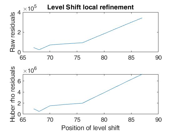
lshiftlocref=struct;
% Set window length for local refinement.
lshiftlocref.wlength=10;
% Set tuning constant to use insde Huber rho function
lshiftlocref.huberc=1.5;
% Estimate the parameters
[out]=LTSts(y1,'model',model,'nsamp',500,...
'plots',1,'lshiftlocref',lshiftlocref,'msg',0);
% Using the notation of the paper RPRH: A=2, B=4, G=2 and $\delta_1>0$.
str=strcat('A=2, B=4, G=2, $\delta_2=',num2str(out.posLS),'$');
numpar = {'model parameters:' , str};
axeslast=findobj('-regexp','Tag','LTSts:ts');
title(axeslast(end),numpar,'interpreter','LaTeX','FontSize',16);
% generate the wedgeplot
% wedgeplot(out,'transpose',true,'extradata',[y1 out.yhat]);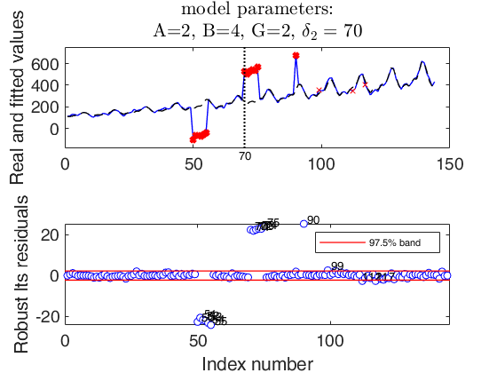

Click here for the graphical output of this example (link to Ro.S.A. website)

Example 2 used in the paper RPRH.

A persisting level shift and three isolated outliers, two of which in proximity of the level shift.

% Load airline data.
%   1949 1950 1951 1952 1953 1954 1955 1956 1957 1958 1959 1960
y = [112  115  145  171  196  204  242  284  315  340  360  417    % Jan
118  126  150  180  196  188  233  277  301  318  342  391    % Feb
132  141  178  193  236  235  267  317  356  362  406  419    % Mar
129  135  163  181  235  227  269  313  348  348  396  461    % Apr
121  125  172  183  229  234  270  318  355  363  420  472    % May
135  149  178  218  243  264  315  374  422  435  472  535    % Jun
148  170  199  230  264  302  364  413  465  491  548  622    % Jul
148  170  199  242  272  293  347  405  467  505  559  606    % Aug
136  158  184  209  237  259  312  355  404  404  463  508    % Sep
119  133  162  191  211  229  274  306  347  359  407  461    % Oct
104  114  146  172  180  203  237  271  305  310  362  390    % Nov
118  140  166  194  201  229  278  306  336  337  405  432 ]; % Dec
close all
y1=y(:);
y1(68:end)=y1(68:end)+1300;
y1(67)=y1(67)-600;
y1(45)=y1(45)-800;
y1(68:69)=y1(68:69)+800;
% Create structure specifying model
model=struct;
model.trend=2;                  % quadratic trend
model.s=12;                     % monthly time series
model.seasonal=204;             % number of harmonics
model.lshift=41:length(y1)-40;  % position where monitoring level shift
model.X=[];
% Create structure lts specifying lts options
lshiftlocref=struct;
% Set window length for local refinement.
lshiftlocref.wlength=10;
% Set tuning constant to use insde Huber rho function
lshiftlocref.huberc=1.5;
% Estimate the parameters
[out, varargout]=LTSts(y1,'model',model,'nsamp',500,...
'plots',1,'lshiftlocref',lshiftlocref,'msg',0);
% Using the notation of the paper RPRH: A=2, B=4, G=2 and $\delta_1>0$.
str=strcat('A=2, B=4, G=2, $\delta_2=',num2str(out.posLS),'$');
numpar = {'model parameters:' , str};
title(findobj('-regexp','Tag','LTSts:ts'),numpar,'interpreter','LaTeX','FontSize',16);
% generate the wedgeplot
% wedgeplot(out,'transpose',true,'extradata',[y1 out.yhat]);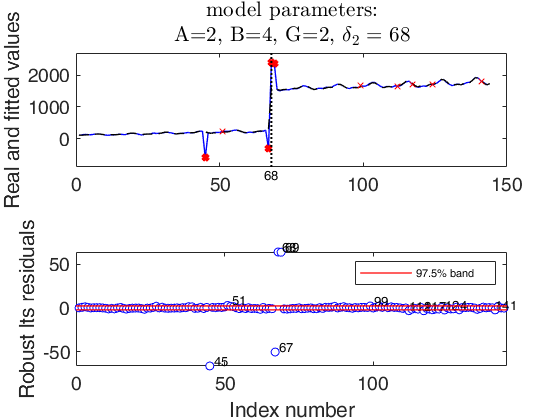

Example 3 used in the paper RPRH.

A persisting level shift preceded and followed in the proximity by other two short level shifts, and an isolated outlier.

% Load airline data.
%   1949 1950 1951 1952 1953 1954 1955 1956 1957 1958 1959 1960
y = [112  115  145  171  196  204  242  284  315  340  360  417    % Jan
118  126  150  180  196  188  233  277  301  318  342  391    % Feb
132  141  178  193  236  235  267  317  356  362  406  419    % Mar
129  135  163  181  235  227  269  313  348  348  396  461    % Apr
121  125  172  183  229  234  270  318  355  363  420  472    % May
135  149  178  218  243  264  315  374  422  435  472  535    % Jun
148  170  199  230  264  302  364  413  465  491  548  622    % Jul
148  170  199  242  272  293  347  405  467  505  559  606    % Aug
136  158  184  209  237  259  312  355  404  404  463  508    % Sep
119  133  162  191  211  229  274  306  347  359  407  461    % Oct
104  114  146  172  180  203  237  271  305  310  362  390    % Nov
118  140  166  194  201  229  278  306  336  337  405  432 ]; % Dec
y1=y(:);
y1(50:55)=y1(50:55)-300;
y1(68:end)=y1(68:end)-700;
y1(70:75)=y1(70:75)+300;
y1(90:90)=y1(90:90)+300;
% Create structure specifying model
model=struct;
model.trend=2;                  % quadratic trend
model.s=12;                     % monthly time series
model.seasonal=204;             % number of harmonics
model.lshift=41:length(y1)-40;  % position where monitoring level shift
model.X=[];
% Create structure lts specifying lts options
lshiftlocref=struct;
% Set window length for local refinement.
lshiftlocref.wlength=10;
% Set tuning constant to use insde Huber rho function
lshiftlocref.huberc=1.5;
close all
% Estimate the parameters
[out, varargout]=LTSts(y1,'model',model,'nsamp',500,...
'plots',2,'lshiftlocref',lshiftlocref,'msg',0);
% Using the notation of the paper RPRH: A=2, B=4, G=2 and $\delta_1>0$.
str=strcat('A=2, B=4, G=2, $\delta_2=',num2str(out.posLS),'$');
numpar = {'model parameters:' , str};
title(findobj('-regexp','Tag','LTSts:ts'),numpar,'interpreter','LaTeX','FontSize',16);
% generate the wedgeplot
% wedgeplot(out,'transpose',true,'extradata',[y1 out.yhat]);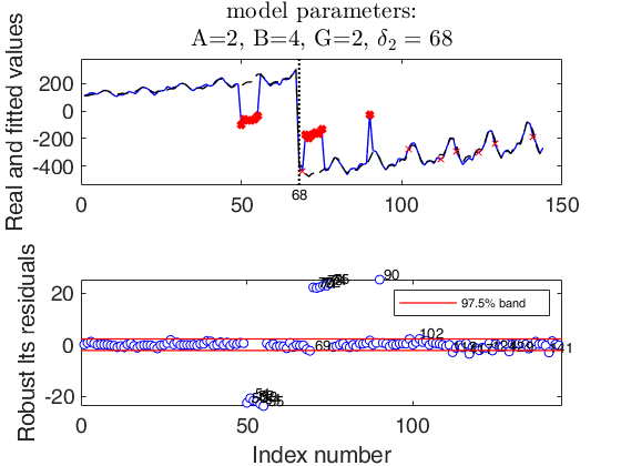

Examples 4 and 5 used in the paper RPRH: trade data.

%% Examples 4 and 5 used in the paper RPRH: trade data.
close all; clear all;
% the datasets
load('TTP12119085');
load('TTP17049075');
Y4 = P12119085{:,1};
Y5 = P17049075{:,1};
% the model
model           = struct;
model.trend     = 1;
model.seasonal  = 102;
model.s         = 12;
model.lshift    = 14:length(Y4)-13;
% LTSts
out4 = LTSts(Y4,'model',model,'plots',0,'dispresults',true,'msg',0);
out5 = LTSts(Y5,'model',model,'plots',0,'dispresults',true,'msg',0);
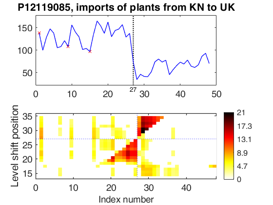
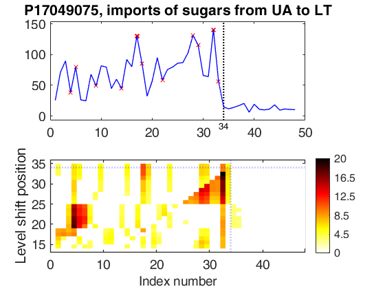
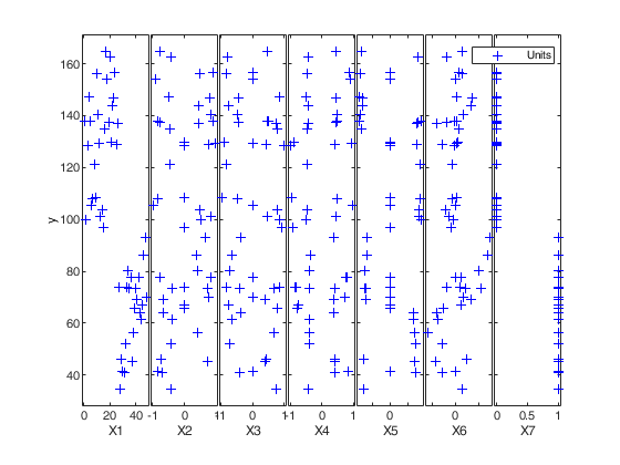
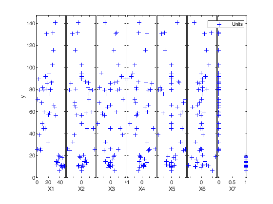
% the wedgeplot with the time series and the detected outliers and
% level shift
wedgeplot(out4,'extradata',Y4,'titl','P12119085, imports of plants from KN to UK');
wedgeplot(out5,'extradata',Y5,'titl','P17049075, imports of sugars from UA to LT');
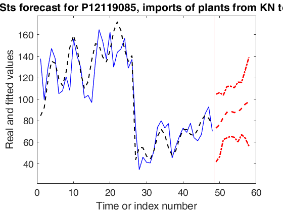
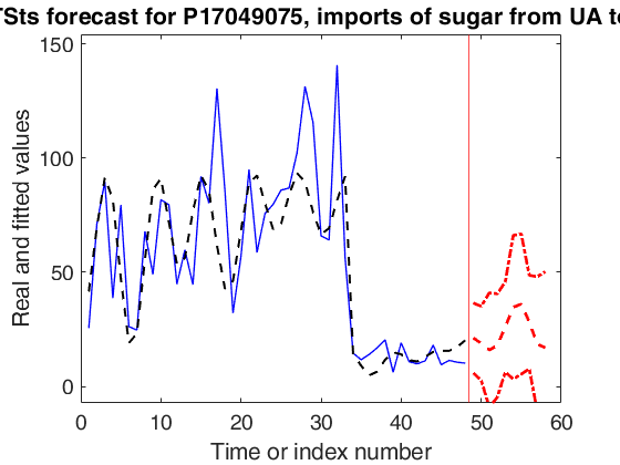
% Forecasts with a 99.9 per cent confidence level
nfore=10;
outfore4 = forecastTS(out4,'model',model,'nfore',nfore,'conflev',0.999,'titl','LTSts forecast for P12119085, imports of plants from KN to UK');
outfore5 = forecastTS(out5,'model',model,'nfore',nfore,'conflev',0.999,'titl','LTSts forecast for P17049075, imports of sugar from UA to LT');
% Comparing with FS (needs conflev option)
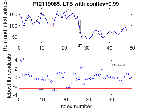
outLTS4 = LTSts(Y4,'model',model,'plots',1,'conflev',0.99,'msg',0);
title(findobj(gcf,'Tag','LTSts:ts'),'P12119085, LTS with conflev=0.99');
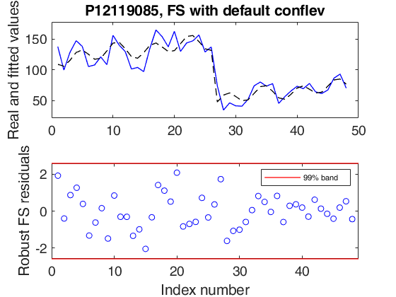
outFRS4 = FSRts(Y4,'model',model,'plots',1);
title(findobj(gcf,'Tag','FSRts:ts'),'P12119085, FS with default conflev');
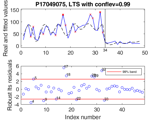
outLTS5 = LTSts(Y5,'model',model,'plots',1,'conflev',0.99,'msg',0);
title(findobj(gcf,'Tag','LTSts:ts'),'P17049075, LTS with conflev=0.99');
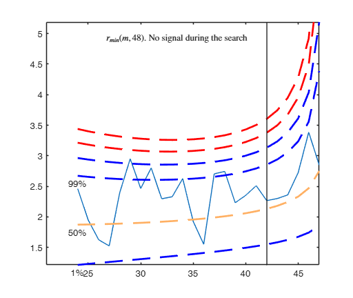
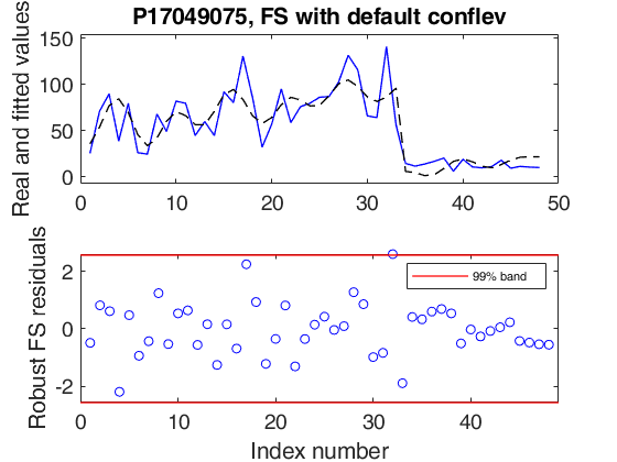
outFRS5 = FSRts(Y5,'model',model,'plots',1);
title(findobj(gcf,'Tag','FSRts:ts'),'P17049075, FS with default conflev');

                  Coeff         SE           t           pval   
                _________    _________    ________    __________

    b_trend1       115.27       4.5051      25.586    2.0728e-26
    b_trend2        1.592      0.27465      5.7965    9.1325e-07
    b_cos1        -2.8294       3.9154    -0.72265        0.4741
    b_sin1        -12.419       4.6909     -2.6475      0.011544
    b_cos2        -9.0708       4.6584     -1.9472      0.058559
    b_sin2        -22.604       4.7099     -4.7992    2.2402e-05
    b_varaml    -0.015796    0.0042445     -3.7215    0.00060891
    b_lshift      -112.62       7.6319     -14.756    8.9212e-18

Level shift position t=27
                  Coeff         SE           t          pval   
                _________    _________    _______    __________

    b_trend1        55.14       3.8549     14.304    2.5537e-17
    b_trend2      0.89673      0.19848     4.5181    5.4202e-05
    b_cos1         15.545       4.1497     3.7461    0.00056646
    b_sin1          3.612       4.2659    0.84671        0.4022
    b_cos2        -32.496       4.2541    -7.6387    2.4573e-09
    b_sin2        -16.057        4.313    -3.7229    0.00060638
    b_varaml    -0.022594    0.0018596     -12.15    5.2846e-15
    b_lshift      -79.413       5.6981    -13.937    6.0952e-17

Level shift position t=34
Level shift for t=14
Level shift for t=15
Level shift for t=16
Level shift for t=17
Level shift for t=18
Level shift for t=19
Level shift for t=20
Level shift for t=21
Level shift for t=22
Level shift for t=23
Level shift for t=24
Level shift for t=25
Level shift for t=26
Level shift for t=27
Level shift for t=28
Level shift for t=29
Level shift for t=30
Level shift for t=31
Level shift for t=32
Level shift for t=33
Level shift for t=34
Level shift for t=35
-------------------------
Signal detection loop
Sample seems homogeneous, no outlier has been found
Summary of the exceedances
           1          99         999        9999       99999
           1           2           0           0           0

Level shift for t=14
Level shift for t=15
Level shift for t=16
Level shift for t=17
Level shift for t=18
Level shift for t=19
Level shift for t=20
Level shift for t=21
Level shift for t=22
Level shift for t=23
Level shift for t=24
Level shift for t=25
Level shift for t=26
Level shift for t=27
Level shift for t=28
Level shift for t=29
Level shift for t=30
Level shift for t=31
Level shift for t=32
Level shift for t=33
Level shift for t=34
Level shift for t=35
-------------------------
Signal detection loop
Sample seems homogeneous, no outlier has been found
Summary of the exceedances
           1          99         999        9999       99999
           0           5           1           0           0

Input Arguments

expand all

`y` — Time series to analyze. Vector.

A row or a column vector with T elements, which contains the time series. Note that y may contain missing values.

Data Types: single| double

Name-Value Pair Arguments

Specify optional comma-separated pairs of Name,Value arguments. Name is the argument name and Value is the corresponding value. Name must appear inside single quotes (' '). You can specify several name and value pair arguments in any order as Name1,Value1,...,NameN,ValueN.

Example:

 'bdp',0.4
, 'conflev',0.99
, 'dispresults',true
, 'h',round(n*0.75)
, 'intercept',false
, 'lshiftlocref',lshiftlocref.typeres=2
, 'lts',lts
, 'model', model
, 'msg',true
, 'nbestindexes',5
, 'nocheck',true
, 'nsamp',500
, 'refstepsALS',20
, 'reftolALS',1e-05
, 'SmallSampleCor',3
, 'yxsave',1
, 'plots',1

`bdp` —breakdown point.scalar.

It measures the fraction of outliers the algorithm should resist. In this case any value greater than 0 but smaller or equal than 0.5 will do fine. Please specify h or bdp, but not both.

Example: 'bdp',0.4

Data Types: double

`conflev` —Confidence level.scalar.

Scalar between 0 and 1 containing Confidence level which is used to declare units as outliers. Usually conflev=0.95, 0.975 0.99 (individual alpha) or 1-0.05/n, 1-0.025/n, 1-0.01/n (simultaneous alpha). Default value is 0.975.

Example: 'conflev',0.99

Data Types: double

`dispresults` —Display results of final fit.boolean.

If dispresults is true, labels of coefficients, estimated coefficients, standard errors, tstat and p-values are shown on the screen in a fully formatted way. The default value of dispresults is false.

Example: 'dispresults',true

Data Types: logical

`h` —The number of observations that determined the least trimmed squares estimator.scalar.

h is an integer greater than p (number of columns of matrix X including the intercept but smaller then n. If the purpose is outlier detection than h does not have to be smaller than [0.5*(T+p+1)]. The default value of h is [0.75*T]. Note that if h is supplied input argument bdp is ignored.

Example: 'h',round(n*0.75)

Data Types: double

`intercept` —Indicator for constant term.true (default) | false.

Indicator for the constant term (intercept) in the fit, specified as the comma-separated pair consisting of 'Intercept' and either true to include or false to remove the constant term from the model.

Example: 'intercept',false

Data Types: boolean

`lshiftlocref` —Parameters for local shift refinement.structure.

This option is used just if model.lshift is greater then 0.

In order to precisely identify level shift position it is necessary to consider a local sum of squares varying the position of the level shift around the first tentative position keeping all the other parameters fixed. This structure contains the following fields:

Value	Description
`wlength`	scalar greater than 0 which identifies the length of the window. The default value is 15, that is the tentative level shift position varies from tl-15, tl-15, ..., tl+14, tl+15, where tl is the best preliminary tentative level shift position.
`typeres`	scalar which identifies the type of residuals to consider. If typerres =1, the local residuals sum of squares is based on huberized (scaled) residuals (this is the default choice) else raw residuals are used.
`huberc`	tuning constant for Huber estimator just in case lshiftlocref.typeres=1. The default value is 2.

Example: 'lshiftlocref',lshiftlocref.typeres=2

Data Types: struct

`lts` —structure which controls a set of options of the maximization procedure.structure.

Structure with the following fields:

Value	Description
`bestr`	scalar defining number of "best betas" to remember from the subsamples. These will be later iterated until convergence. The default is 20 (10 of them are the best from previous iteration in case a level shift is present).
`refsteps`	scalar defining number of concentration steps (default = 2). refsteps = 0 means "raw-subsampling" without iterations.
`refstepsbestr`	scalar defining maximum number of refining steps for each best subset (default=50).
`reftol`	scalar. Default value of tolerance for the refining steps The default value is 1e-6;
`reftolbestr`	scalar. Default value of tolerance for the refining steps for each of the best subsets The default value is 1e-8. Remark: if lts is an empty value all default values of structure lts will be used.

Example: 'lts',lts

Data Types: struct

`model` —model type.structure.

A structure which specifies the model which will be used. The model structure contains the following fields:

Value	Description
`s`	scalar (length of seasonal period). For monthly data s=12 (default), for quartely data s=4, ...
`trend`	scalar (order of the trend component). trend = 0 implies no trend; trend = 1 implies linear trend with intercept (default); trend = 2 implies quadratic trend; trend = 3 implies cubic trend. Admissible values for trend are, 0, 1, 2 and 3. In the paper RPRH to denote the order of the trend symbol A is used.
`seasonal`	scalar (integer specifying number of frequencies, i.e. harmonics, in the seasonal component. Possible values for seasonal are $0,1, 2, ..., [s/2]$, where $[s/2]=floor(s/2)$. If seasonal =0 we assume there is no seasonal component. If seasonal =1 (default) we have: $\beta_1 \cos( 2 \pi t/s) + \beta_2 sin ( 2 \pi t/s)$; if seasonal =2 we have: $\beta_1 \cos( 2 \pi t/s) + \beta_2 \sin ( 2 \pi t/s) + \beta_3 \cos(4 \pi t/s) + \beta_4 \sin (4 \pi t/s)$. Note that when $s$ is even the sine term disappears for $j=s/2$ and so the maximum number of trigonometric parameters is $s-1$. If seasonal is a number greater than 100 then it is possible to specify how the seasonal component grows over time. For example, seasonal = 101 implies a seasonal component which just uses one frequency which grows linearly over time as follows: $(1+\beta_3 t)\times ( \beta_1 cos( 2 \pi t/s) + \beta_2 \sin ( 2 \pi t/s))$. For example, seasonal =201 implies a seasonal component which just uses one frequency which grows in a quadratic way over time as follows: $(1+\beta_3 t + \beta_4 t^2)\times( \beta_1 \cos( 2 \pi t/s) + \beta_2 \sin ( 2 \pi t/s))$. seasonal =0 implies a non seasonal model. In the paper RPRH to denote the number of frequencies of the seasonal component symbol B is used, while symbol G is used to denote the order of the trend of the seasonal component. Therefore, for example, model.seasonal=201 corresponds to B=1 and G=2, while model.seasonal=3 corresponds to B=3 and G=0;
`X`	matrix of size T-by-nexpl containing the values of nexpl extra covariates which are likely to affect y.
`lshift`	scalar or vector associated to level shift component. lshift=0 (default) implies no level shift component. If model.lshift is vector of positive integers, then it is associated to the positions of level shifts which have to be considered. The most significant one is included in the fitted model. For example if model.lshift =[13 20 36] a tentative level shift is imposed in position $t=13$, $t=20$ and $t=36$. The most significant among these positions in included in the final model. In other words, the following extra parameters are added to the final model: $\beta_{LS1}* I(t \geq \beta_{LS2})$ where $\beta_{LS1}$ is a real number (associated with the magnitude of the level shift) and $\beta_{LS2}$ is an integer which assumes values 13, 20 or 36 and and $I$ denotes the indicator function. As a particular case, if model.lshift =13 then a level shift in position $t=13$ is added to the model. In other words the following additional parameters are added: $\beta_{LS1}* I(t \geq 13)$ where $\beta_{LS1}$ is a real number and $I$ denotes the indicator function. If lshift = -1 tentative level shifts are considered for positions $p+1,p+2, ..., T-p$ and the most significant one is included in the final model ($p$ is the total number of parameters in the fitted model). Note that lshift=-1 is not supported for C-coder translation. In the paper RPRH $\beta_{LS1}$ is denoted with symbol $\delta_1$, while, $\beta_{LS2}$ is denoted with symbol $\delta_2$.
`ARp`	vector with non negative integer numbers specifying the autoregressive components. For example: model.ARp=[1 2] means a AR(2) process; model.ARp=2 means just the lag 2 component; model.ARp=[1 2 5 8] means AR(2) + lag 5 + lag 8; model.ARp=0 (default) means no autoregressive component.
`ARtentout`	matrix of size r-by-2 containing the list of the units declared as outliers (first column) and corresponding fitted values (second column) or empty scalar. If model.ARtentout is not empty, when the autoregressive component is present, the y values which are used to compute the autoregressive component are replaced by model.tentout(:,2) for the units contained in model.tentout(:,1) Remark: the default model is for monthly data with a linear trend (2 parameters) + seasonal component with just one harmonic (2 parameters), no additional explanatory variables and no level shift that is model=struct; model.s=12; model.trend=1; model.seasonal=1; model.X=[]; model.lshift=0; Using the notation of the paper RPRH we have A=1, B=1; and $\delta_1=0$.

Example: 'model', model

Data Types: struct

`msg` —Messages on the screen.boolean.

Scalar which controls whether to display or not messages on the screen. If msg==true (default) messages are displayed on the screen about estimated time to compute the estimator and the warnings about 'MATLAB:rankDeficientMatrix', 'MATLAB:singularMatrix' and 'MATLAB:nearlySingularMatrix' are set to off else no message is displayed on the screen

Example: 'msg',true

Data Types: logical

`nbestindexes` —position of the best solutions.positive integer.

For each tentative level shift solution, it is interesenting to understand whether best solutions of target function come from subsets associated with current level shift solution or from best solutions from previous tentative level shift position. The indexes from 1 to lts.bestr/2 are associated with subsets just extracted. The indexes from lts.bestr/2+1 to lts.bestr are associated with best solutions from previous tentative level shift. More precisely: index lts.bestr/2+1 is associated with best solution from previous tentative level shift;

index lts.bestr/2+2 is associated with second best solution from previous tentative level shift;

...

nbestindexes is an integer which specifies how many indexes we want to store. The default value of nbestindexes is 3.

Example: 'nbestindexes',5

Data Types: double

`nocheck` —Check input arguments.boolean.

If nocheck is equal to true no check is performed on matrix y and matrix X. Notice that y and X are left unchanged. In other words the additioanl column of ones for the intercept is not added. As default nocheck=false. The controls on h, bdp and nsamp still remain.

Example: 'nocheck',true

Data Types: boolean

`nsamp` —number of subsamples to extract.scalar | vector of length 2.

Vector of length 1 or 2 which controls the number of subsamples which will be extracted to find the robust estimator. If lshift is not equal to 0 then nsamp(1) controls the number of subsets which have to be extracted to find the solution for t=lshift(1). nsamp(2) controls the number of subsets which have to be extracted to find the solution for t=lshift(2), lshift(3), ..., lshift(end).

Note that nsamp(2) is generally smaller than nsamp(1) because in order to compute the best solution for t=lshift(2), lshift(3), ..., lshift(end), we use the lts.bestr/2 best solutions from previous t (after shifting the position of the level shift in the estimator of beta). If lshift is a vector of positive integers the default value of nsamp is (500 250). If lshift is a vector of positive integers and nsamp is supplied as a scalar the default is to extract [nsamp/2] subsamples for t=lshift(1), lshift(2), ... Therefore, for example, in order to extract 600 subsamples for t=lshift(1) and 300 subsamples for t= lshift(2) ... you can use nsamp =600 or nsamp=[600 300].

The default value of nsamp is 1000;

Remark: if nsamp=0 all subsets will be extracted.

They will be (n choose p).

Example: 'nsamp',500

Data Types: double

`refstepsALS` —Maximum iterations inside ALS.scalar.

Maximum number of iterations inside ALS routine. Default value of tolerance for the refining steps inside ALS routine. The default value is 50.

Example: 'refstepsALS',20

Data Types: double

`reftolALS` —Tolerance inside ALS.scalar.

Tolerance value of tolerance for the refining steps inside ALS routine. The default value is 1e-03.

Example: 'reftolALS',1e-05

Data Types: double

`SmallSampleCor` —Small sample correction factor to control empirical size of the test.scalar equal to 1 | 2 (default) | 3 | 4.

- If SmallSampleCor=1 in the reweighting step the nominal threshold based on $\chi^2_{0.99}$ is multiplied by the small sample correction factor which guarrantees that the empirical size of the test is equal to the nominal size.

Given that the correction factors were obtained through simulation for a linear model, the number of explanatory which is used to compute the correction factor refers to all explanatory variables except the non linear components in the seasonal part of the model. For example, in a model with linear trend 4 seasonal harmonics + level shift and second order trend in the seasonal component the number of explanatory variables used is 11 = total number of variables -2 = 2 (linear trend) + 8 (4 seasonal harmonics) +1 (level shift).

- If SmallSampleCor =2 Gervini and Yohai procedure is called with 'iterating' false and 'alpha' 0.99 is invoked, that is: weights=GYfilt(stdres,'iterating',false,'alpha',0.99);

- If SmallSampleCor =3 Gervini and Yohai procedure called with 'iterating' true and 'alpha' 0.99 is invoked, that is: weights=GYfilt(stdres,'iterating',true,'alpha',0.99);

- If SmallSampleCor =4 $\chi^2_{0.99}$ threshold is used that is: weights = abs(stdres)<=sqrt(chi2inv(0.99,1));

Example: 'SmallSampleCor',3

Data Types: double

`yxsave` —store X and y.boolean.

Scalar that is set to 1 to request that the response vector y and data matrix X are saved into the output structure out.

Default is 0, i.e. no saving is done.

Example: 'yxsave',1

Data Types: logical

`plots` —Plots on the screen.scalar.

If plots = 1, a two panel plot will be shown on the screen.

The upper panel contains the orginal time series with fitted values. The bottom panel will contain the plot of robust residuals against index number. The confidence level which is used to draw the horizontal lines associated with the bands for the residuals is specified in input option conflev. If conflev is missing a nominal 0.975 confidence interval will be used. If plots =2 the following additional plots will be shown on the screen.

1) Boxplot of the distribution of the lts.bestr values of the target function for each tentative level shift position;

2) A two panel plot which shows the values of the local sum of squares varying the position of the level shift around the first tentative position keeping all the other parameters fixed. Top panel refers to Huberized residuals sum of squares and bottom panel refers to residual sum of squares.

3) A plot which shows the indexes of the best nbestindexes solutions for each tentative level shift position.

4) A plot which shows the relative frequency of inclusion of each unit in the best h-subset after lts.refsteps refining steps.

5) A plot which shows the relative frequency of inclusion of each unit inside the best nbestindexes subsets which are brought to full convergence.

The default value of plot is 0 i.e. no plot is shown on the screen.

Example: 'plots',1

Data Types: double

Output Arguments

expand all

`out` — description Structure

A structure containing the following fields

Value	Description
`B`	Matrix containing estimated beta coefficients, (including the intercept when options.intercept=true) standard errors, t-stat and p-values The content of matrix B is as follows: 1st col = beta coefficients The order of the beta coefficients is as follows: 1) trend elements (if present). If the trend is of order two there are r+1 coefficients if the intercept is present otherwise there are just r components; 2) linear part of seasonal component 2, 4, 6, ..., s-2, s-1 coefficients (if present); 3) coefficients associated with the matrix of explanatory variables which have a potential effect on the time series under study (X or autoregressive part); If model.ARp>0 the first model.ARp elements refer to the autoregressive component. 4) non linear part of seasonal component, that is varying amplitude. If varying amplitude is of order k there are k coefficients (if present); 5) level shift component (if present). In out.B it is shown just the real number which identifies the magnitude of the upward (downward) level shift. The integer which specifies the time in which level shift takes place is given in output out.posLS. 2nd col = standard errors; 3rd col = t-statistics; 4th col = p values.
`Btable`	same thing as out.B but in table format.
`h`	The number of observations that have determined the initial LTS estimator, i.e. the value of h.
`bs`	Vector containing the units with the smallest p+k squared residuals before the reweighting step, where p is the total number of the parameters in the model and p+k is smallest number of units such that the design matrix is full rank. out.bs can be used to initialize the forward search.
`Hsubset`	matrix of size T-by-r containing units forming best H subset for each tentative level shift which is considered. r is number of tentative level shift positions whicha re considered. For example if model.lshift=[13 21 40] r is equal to 3. Units belonging to subset are given with their row number, units not belonging to subset have missing values This output is present just if input option model.lshift is not equal to 0.
`lshift`	(row) vector containing level shift positions which have been tested. out.lshift =0 means that level position has not been investigated.
`posLS`	scalar associated with best tentative level shift position. This output is present just if input option model.lshift is not equal to 0.
`numscale2`	matrix of size lts.bestr-by-(T-2*lshift) containing (in the columns) the values of the lts.bestr smallest values of the target function. Target function = truncated residuals sum of squares.
`BestIndexes`	matrix of size nbestindexes-by-(T-2*lshift) containing in each column the indexes associated with the best nbestindexes solutions. The indexes from lts.bestr/2+1 to lts.bestr are associated with best solutions from previous tentative level shift. More precisely: index lts.bestr/2+1 is associated with best solution from previous tentative level shift; index lts.bestr/2+2 is associated with best solution from previous tentative level shift. This output is present just if input option model.lshift is not equal to 0.
`Likloc`	matrix of size (2*lshiftlocref.wlength+1)-by-3 containing local sum of squares of residuals in order to decide best position of level shift: 1st col = position of level shift; 2nd col = local sum of squares of huberized residuals; 3rd col = local sum of squares of raw residuals. This output is present just if input option model.lshift is not equal to 0.
`RES`	Matrix of size T-by-(T-lshift) containing scaled residuals for all the T units of the original time series monitored in steps lshift+1, lshift+2, ..., T-lshift, where lshift+1 is the first tentative level shift position, lshift +2 is the second level shift position, and so on. This output is present just if input option model.lshift is not equal to 0.
`yhat`	vector of fitted values after final (NLS=non linear least squares) step. $ (\hat \eta_1, \hat \eta_2, \ldots, \hat \eta_T)'$
`residuals`	Vector T-by-1 containing the scaled residuals from after final NLS step.
`weights`	Vector containing weights after adaptive reweighting. The elements of this vector are 0 or 1. These weights identify the observations which are used to compute the final NLS estimate.
`scale`	Final scale estimate of the residuals using final weights. \[ \hat \sigma = cor \times \sum_{i \in S_m} [y_i- \eta(x_i,\hat \beta)]^2/(m-p) \] where $S_m$ is a set of cardinality $m$ which contains the units not declared as outliers, $p$ is the total number of estimated parameters and $cor$ is a correction factor to make the estimator consistent.
`conflev`	confidence level which is used to declare outliers. Remark: scalar out.conflev will be used to draw the horizontal lines (confidence bands) in the plots
`outliers`	vector containing the list of the units declared as outliers using confidence level specified in input scalar conflev.
`outliersPval`	p-value of the units declared as outliers.
`singsub`	Number of subsets wihtout full rank. Notice that if this number is greater than 0.1*(number of subsamples) a warning is produced on the screen
`invXX`	$cov(\beta)/\hat \sigma^2$. p-by-p, square matrix. If the model is linear out.invXX is equal to $(X'X)^{-1}$, else out.invXX is equal to $(A'A)^{-1}$ where $A$ is the matrix of partial derivatives. More precisely: \[ a_{i,j}=\frac{\partial \eta_i(x_i, \hat \beta)}{\partial \hat \beta_j} \] where \begin{eqnarray} y_i & = & \eta(x_i,\beta)+ \epsilon_i \\ & = & \eta_i +\epsilon_i \\ & = & \eta(x_i,\hat \beta)+ e_i \\ & = & \hat \eta_i + e_i \end{eqnarray}
`LastHarmonicPval`	combined p value for the two coefficients of the last harmonic (this p value comes from an F test).
`LevelShiftPval`	p value of the level shift which takes into account (this pvalue comes from Bonferronization to take it account that if you impose a level shift, this component is always found).
`y`	response vector y.
`X`	data matrix X containing trend, seasonal, expl (with autoregressive component) and lshift, if the model is linear or linearized version of $\eta(x_i, \beta)$ if the model is non linear containing in the columns partial derivatives evaluated in correspondence of out.B(:,1) with respect to each parameter. In other words, the $i,j$-th element of out.X is \[ \frac{\partial \eta_i(x_i, \hat \beta)}{\partial \hat \beta_j} \] $j=1, 2, \ldots, p$, $i \in S_m$. The size of this matrix is: n-length(out.outliers)-by-p The field is present only if option yxsave is set to 1.
`class`	'LTSts'.

`varargout` —Indices of the subsamples extracted for computing the estimate (the so called elemental sets) for each tentative level shift position. C : cell

C{1} is associated with the subsamples for first tentative level shift position;

C{2} is associated with the subsamples for second tentative level shift position;

...

C{end} is associated with the subsamples for last tentative level shift position;

References

Rousseeuw, P.J., Perrotta D., Riani M. and Hubert, M. (2018), Robust Monitoring of Many Time Series with Application to Fraud Detection, "Econometrics and Statistics". [RPRH]

LTSts

Syntax

Description

Examples

Related Examples

Input Arguments

y — Time series to analyze. Vector.

Name-Value Pair Arguments

bdp —breakdown point.scalar.

conflev —Confidence level.scalar.

dispresults —Display results of final fit.boolean.

h —The number of observations that determined the least trimmed squares estimator.scalar.

intercept —Indicator for constant term.true (default) | false.

lshiftlocref —Parameters for local shift refinement.structure.

lts —structure which controls a set of options of the maximization procedure.structure.

model —model type.structure.

msg —Messages on the screen.boolean.

nbestindexes —position of the best solutions.positive integer.

nocheck —Check input arguments.boolean.

nsamp —number of subsamples to extract.scalar | vector of length 2.

refstepsALS —Maximum iterations inside ALS.scalar.

reftolALS —Tolerance inside ALS.scalar.

SmallSampleCor —Small sample correction factor to control empirical size of the test.scalar equal to 1 | 2 (default) | 3 | 4.

yxsave —store X and y.boolean.

plots —Plots on the screen.scalar.

Output Arguments

out — description Structure

varargout —Indices of the subsamples extracted for computing the estimate (the so called elemental sets) for each tentative level shift position. C : cell

References

See Also

`y` — Time series to analyze. Vector.

`bdp` —breakdown point.scalar.

`conflev` —Confidence level.scalar.

`dispresults` —Display results of final fit.boolean.

`h` —The number of observations that determined the least trimmed squares estimator.scalar.

`intercept` —Indicator for constant term.true (default) | false.

`lshiftlocref` —Parameters for local shift refinement.structure.

`lts` —structure which controls a set of options of the maximization procedure.structure.

`model` —model type.structure.

`msg` —Messages on the screen.boolean.

`nbestindexes` —position of the best solutions.positive integer.

`nocheck` —Check input arguments.boolean.

`nsamp` —number of subsamples to extract.scalar | vector of length 2.

`refstepsALS` —Maximum iterations inside ALS.scalar.

`reftolALS` —Tolerance inside ALS.scalar.

`SmallSampleCor` —Small sample correction factor to control empirical size of the test.scalar equal to 1 | 2 (default) | 3 | 4.

`yxsave` —store X and y.boolean.

`plots` —Plots on the screen.scalar.

`out` — description Structure

`varargout` —Indices of the subsamples extracted for computing the estimate (the so called elemental sets) for each tentative level shift position. C : cell