
|
LTSts |
LTStsVarSel |
 |
LTStsLSmult
LTStsLSmult extends LTSts to the detection of multiple Level Shifts in time series
Description
Examples
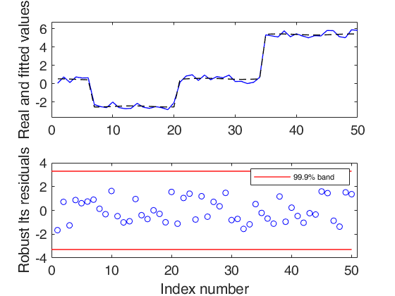
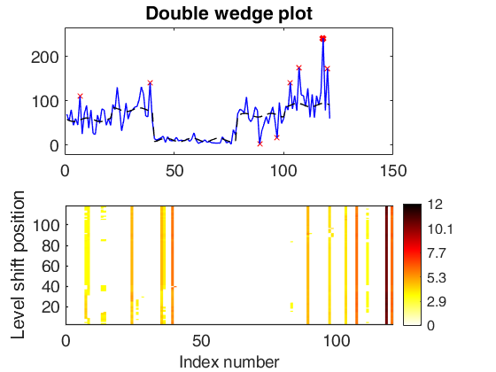
 A synthetic example with optional arguments msg and plots.
A synthetic example with optional arguments msg and plots.
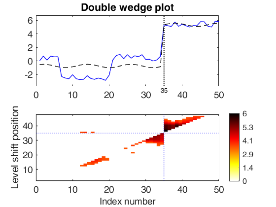
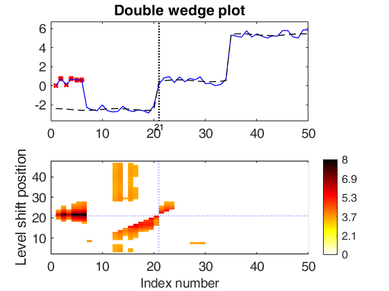
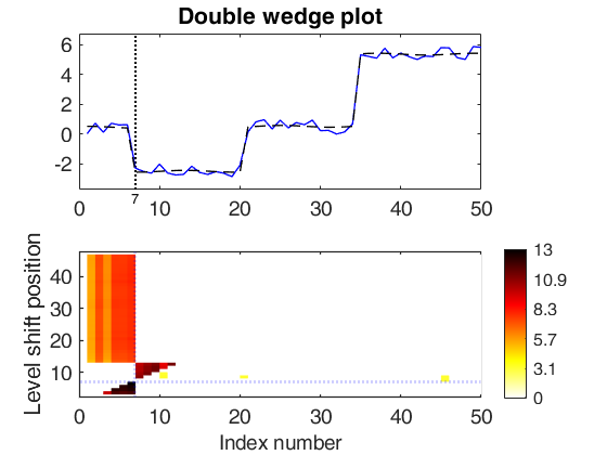
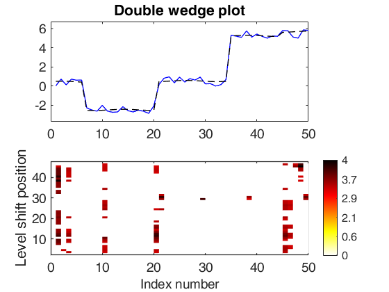
Y=rand(50,1);
Y(35:end)=Y(35:end)+5;
Y(7:20)=Y(7:20)-3;
out  = LTStsLSmult(Y,'msg',true,'plots',1);
significant LS at position 35 (pval = 7.1054e-15)
significant LS at position 21 (pval = 0)
significant LS at position 7 (pval = 0)

Related Examples
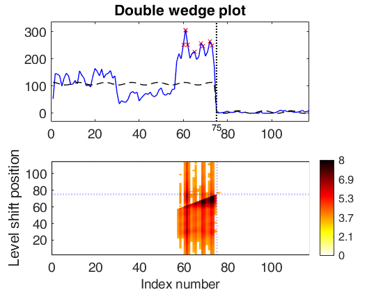
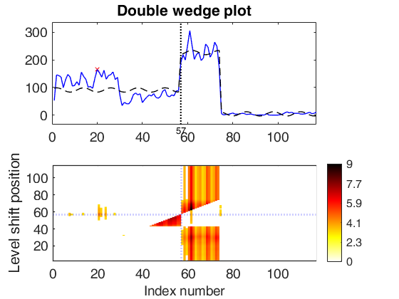
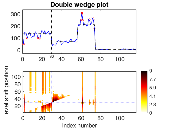
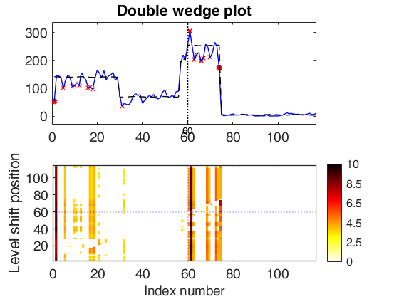
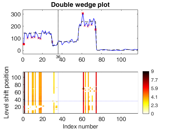
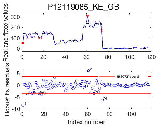
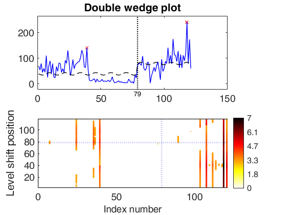
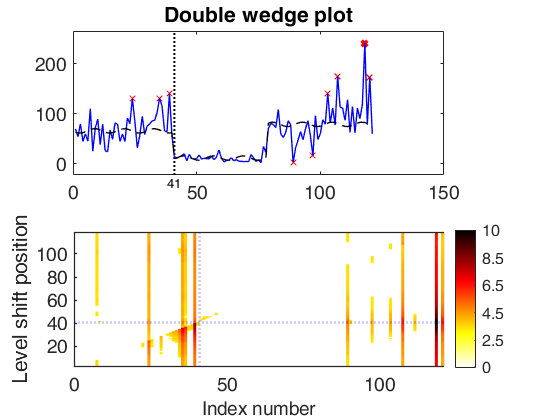
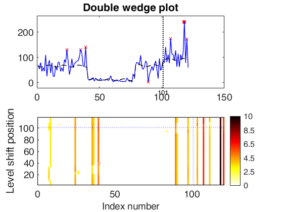
Trade data examples.
Trade data examples.Two examples taken from the (extended version of the) series in: Rousseeuw, P.J., Perrotta D., Riani M. and Hubert, M. (2018), Robust Monitoring of Many Time Series with Application to Fraud Detection, "Econometrics and Statistics".
load TTplant  % KE-GB
load TTsugar   % UA-LT
yin1   = plant{:,1};
yin2   = sugar{:,1};
out1  = LTStsLSmult(yin1,'msg',true,'plots',1);
sgtitle('P12119085_KE_GB','interpreter','none','Fontsize',20);
pause(1);
out2  = LTStsLSmult(yin2,'msg',true,'plots',1);
sgtitle('P17049075_UA_LT','interpreter','none','Fontsize',20);
significant LS at position 75 (pval = 0)
significant LS at position 57 (pval = 0)
significant LS at position 30 (pval = 0)
significant LS at position 60 (pval = 0)
significant LS at position 36 (pval = 1.7337e-10)
significant LS at position 79 (pval = 4.793e-06)
significant LS at position 41 (pval = 0)
significant LS at position 101 (pval = 0.0096827)
Input Arguments
Output Arguments
References
Rousseeuw, P.J., Perrotta D., Riani M. and Hubert, M. (2018), Robust Monitoring of Many Time Series with Application to Fraud Detection, "Econometrics and Statistics". [RPRH]
See Also
|
|
LTSts |
LTStsVarSel |
|
|
|
Functions |
|
• The developers of the toolbox • The forward search group • Terms of Use • Acknowledgments