MMreg

MMreg computes MM estimator of regression coefficients

Syntax

Description

example

out =MMreg(y, X) MMreg with all default options.

example

out =MMreg(y, X, Name, Value) MMreg with optional input arguments.

example

[out , varargout] =MMreg(___) MMreg with optional input arguments.

Examples

expand all

  • MMreg with all default options.
  • Run this code to see the output shown in the help file

    n=200;
    p=3;
    randn('state', 123456);
    X=randn(n,p);
    % Uncontaminated data
    y=randn(n,1);
    % Contaminated data
    ycont=y;
    ycont(1:5)=ycont(1:5)+6;
    [out]=MMreg(ycont,X);

  • MMreg with optional input arguments.
  • MMreg using the hyperbolic rho function.

    % Run this code to see the output shown in the help file
    n=200;
    p=3;
    randn('state', 123456);
    X=randn(n,p);
    % Uncontaminated data
    y=randn(n,1);
    % Contaminated data
    ycont=y;
    ycont(1:5)=ycont(1:5)+6;
    [out]=MMreg(ycont,X,'Srhofunc','optimal');

  • MMreg with optional input arguments.
  • MMreg using the OLS estimates ac InitialEst.

    % Run this code to see the output shown in the help file
    n=200;
    p=3;
    randn('state', 123456);
    X=randn(n,p);
    % Uncontaminated data
    y=randn(n,1);
    % Contaminated data
    ycont=y;
    ycont(1:5)=ycont(1:5)+6;
    % OLS estimates
    bols=[ones(n,1) X]\y;
    res=y-[ones(n,1) X]*bols;
    sols=sqrt((res'*res)/(n-p-1));
    InitialEst.beta=bols;
    InitialEst.scale=sols;
    [out]=MMreg(ycont,X,'InitialEst',InitialEst);

    Related Examples

    expand all

  • Comparing the output of different MMreg runs.
  • state=100;
    randn('state', state);
    n=100;
    X=randn(n,3);
    bet=[3;4;5];
    y=3*randn(n,1)+X*bet;
    y(1:20)=y(1:20)+13;
    %For outlier detection we consider both the nominal individual 1%
    %significance level and the simultaneous Bonferroni confidence level.
    % Define nominal confidence level
    conflev=[0.99,1-0.01/length(y)];
    % Define number of subsets
    nsamp=3000;
    % Define the main title of the plots
    titl='';
    % MM  estimators
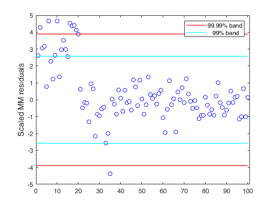
    [outMM]=MMreg(y,X,'conflev',conflev(1));
    laby='Scaled MM residuals';
    resindexplot(outMM.residuals,'title',titl,'laby',laby,'numlab','','conflev',conflev)
    % In this example MM estimator seems to detect half of the outlier with a Bonferroni significance level.
    % By simply changing the seed to 543 (state=543), using a Bonferroni size
    %of 1%, no unit is declared as outlier and just half of them using the 99%
    %band.
    Total estimated time to complete S estimate:  1.01 seconds 
    
    Click here for the graphical output of this example (link to Ro.S.A. website)

  • Comparison between direct call to MMreg and call to Sreg and MMregcore.
  • n=30;
    p=3;
    randn('state', 123456);
    X=randn(n,p);
    % Uncontaminated data
    y=randn(n,1);
    % Contaminated data
    ycont=y;
    ycont(1:5)=ycont(1:5)+6;
    % Two different rho functions are used for S and MM
    rhofuncS='hyperbolic';
    rhofuncMM='hampel';
    % Direct call to MMreg
    [out]=MMreg(ycont,X,'Srhofunc',rhofuncS,'rhofunc',rhofuncMM,'Snsamp',0);
    % Call to Sreg and then to MMregcore
    [outS]=Sreg(ycont,X,'rhofunc',rhofuncS,'nsamp',0);
    outMM=MMregcore(ycont,X,outS.beta,outS.scale,'rhofunc',rhofuncMM);
    disp('Difference between direct call to S and the calls to Sreg and MMregcore')
    max(abs([out.beta-outMM.beta]))

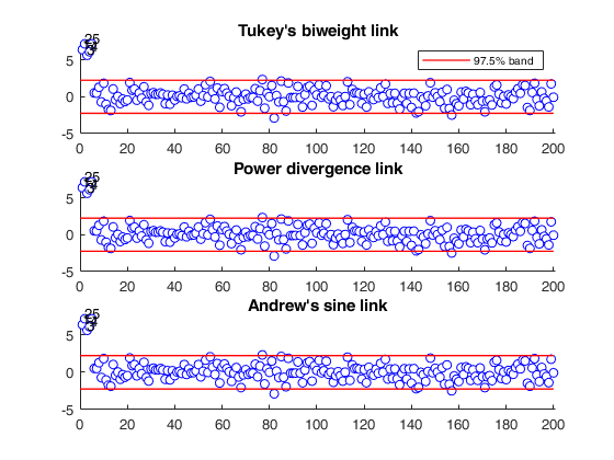
  • Comparison of TB, PD and Andrew's sine estimator.
  • close all
    n=200;
    p=3;
    rng('default')
    rng(100);
    X=randn(n,p);
    % Uncontaminated data
    y=randn(n,1);
    % Contaminated data
    ycont=y;
    ycont(1:5)=ycont(1:5)+6;
    close all
    h1=subplot(3,1,1);
    % TB  is used both in the S and in MM step.
    [outTB]=MMreg(ycont,X,'plots',0);
    resindexplot(outTB,'h',h1)
    title('Tukey''s biweight link')
    % mdpd is used both in the S and in MM step.
    [outmdpd]=MMreg(ycont,X,'Srhofunc','mdpd','rhofunc','mdpd','plots',0);
    h2=subplot(3,1,2);
    resindexplot(outmdpd,'h',h2)
    title('Power divergence link')
    % AS is used both in the S and in MM step.
    [outAS]=MMreg(ycont,X,'Srhofunc','AS','rhofunc','AS','plots',0);
    h3=subplot(3,1,3);
    resindexplot(outAS,'h',h3)
    title('Andrew''s sine link')
    Total estimated time to complete S estimate:  0.90 seconds 
    Total estimated time to complete S estimate:  0.17 seconds 
    Total estimated time to complete S estimate:  0.52 seconds 
    
    Click here for the graphical output of this example (link to Ro.S.A. website)

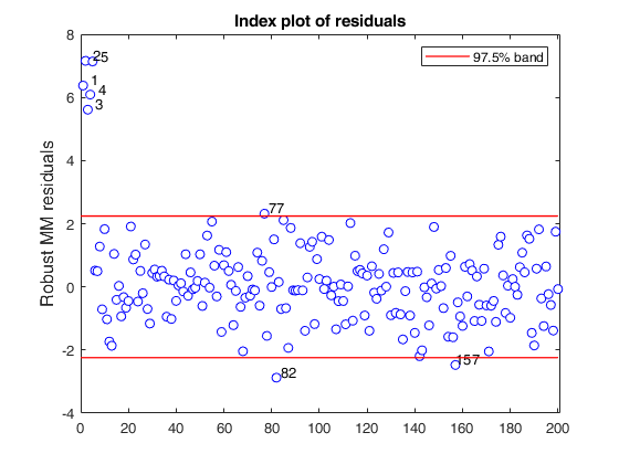
  • Example of the use of Power Divergence estimator.
  • n=200;
    p=3;
    rng('default')
    rng(100);
    X=randn(n,p);
    % Uncontaminated data
    y=randn(n,1);
    % Contaminated data
    ycont=y;
    ycont(1:5)=ycont(1:5)+6;
    % mdpd is used both in the S and in MM step.
    [out]=MMreg(ycont,X,'Srhofunc','mdpd','rhofunc','mdpd','plots',1);
    Total estimated time to complete S estimate:  0.15 seconds 
    
    Click here for the graphical output of this example (link to Ro.S.A. website)

    Input Arguments

    expand all

    y — Response variable. Vector.

    A vector with n elements that contains the response variable. y can be either a row or a column vector.

    Data Types: single| double

    X — Data matrix of explanatory variables (also called 'regressors') of dimension (n x p-1). Rows of X represent observations, and columns represent variables.

    Missing values (NaN's) and infinite values (Inf's) are allowed, since observations (rows) with missing or infinite values will automatically be excluded from the computations.

    Data Types: single| double

    Name-Value Pair Arguments

    Specify optional comma-separated pairs of Name,Value arguments. Name is the argument name and Value is the corresponding value. Name must appear inside single quotes (' '). You can specify several name and value pair arguments in any order as Name1,Value1,...,NameN,ValueN.

    Example: 'conflev',0.99 , 'eff',0.99 , 'effshape',1 , 'InitialEst',[] , 'intercept',false , 'nocheck',true , 'refsteps',10 , 'rhofunc','optimal' , 'rhofuncparam',5 , 'Snsamp',1000 , 'tol',1e-10 , 'yxsave',1 , 'plots',0

    conflev —Confidence level which is used to declare units as outliers.scalar.

    Usually conflev=0.95, 0.975 0.99 (individual alpha) or 1-0.05/n, 1-0.025/n, 1-0.01/n (simultaneous alpha).

    Default value is 0.975

    Example: 'conflev',0.99

    Data Types: double

    eff —nominal efficiency.scalar.

    Scalar defining nominal efficiency (i.e. a number between 0.5 and 0.99). The default value is 0.95 Asymptotic nominal efficiency is: $(\int \psi' d\Phi)^2 / (\psi^2 d\Phi)$

    Example: 'eff',0.99

    Data Types: double

    effshape —location or scale efficiency.dummy scalar.

    If effshape=1 efficiency refers to shape efficiency else (default) efficiency refers to location

    Example: 'effshape',1

    Data Types: double

    InitialEst —starting values of the MM-estimator.[] (default) | structure.

    InitialEst must contain the following fields

    Value Description
    beta

    v x 1 vector (estimate of the initial regression coefficients)

    scale

    scalar (estimate of the scale parameter).

    If InitialEst is empty (default) or InitialEst.beta continas NaN values, program uses S estimators. In this last case it is possible to specify the options given in function Sreg.

    Example: 'InitialEst',[]

    Data Types: struct or empty value

    intercept —Indicator for constant term.true (default) | false.

    Indicator for the constant term (intercept) in the fit, specified as the comma-separated pair consisting of 'Intercept' and either true to include or false to remove the constant term from the model.

    Example: 'intercept',false

    Data Types: boolean

    nocheck —Check input arguments.boolean.

    If nocheck is equal to true no check is performed on matrix y and matrix X. Notice that y and X are left unchanged. In other words the additional column of ones for the intercept is not added.

    As default nocheck=false.

    Example: 'nocheck',true

    Data Types: boolean

    refsteps —Maximum iterations.scalar.

    Scalar defining maximum number of iterations in the MM loop. Default value is 100.

    Example: 'refsteps',10

    Data Types: double

    rhofunc —rho function.string.

    String which specifies the rho function which must be used to weight the residuals.

    Possible values are 'bisquare';

    'optimal';

    'hyperbolic';

    'hampel';

    'mdpd'.

    'AS'.

    'bisquare' uses Tukey's $\rho$ and $\psi$ functions.

    See TBrho and TBpsi.

    'optimal' uses optimal $\rho$ and $\psi$ functions.

    See OPTrho and OPTpsi.

    'hyperbolic' uses hyperbolic $\rho$ and $\psi$ functions.

    See HYPrho and HYPpsi.

    'hampel' uses Hampel $\rho$ and $\psi$ functions.

    See HArho and HApsi.

    'mdpd' uses Minimum Density Power Divergence $\rho$ and $\psi$ functions.

    See PDrho and PDpsi.

    'AS' uses Andrew's sine $\rho$ and $\psi$ functions.

    See ASrho and ASpsi.

    The default is bisquare

    Example: 'rhofunc','optimal'

    Data Types: char

    rhofuncparam —Additional parameters for the specified rho function.scalar | vector.

    For hyperbolic rho function it is possible to set up the value of k = sup CVC (the default value of k is 4.5).

    For Hampel rho function it is possible to define parameters a, b and c (the default values are a=2, b=4, c=8)

    Example: 'rhofuncparam',5

    Data Types: single | double

    Soptions —options to pass to Sreg for initial S estimator.name value pairs.

    Options if initial estimator is S and InitialEst is empty.

    The options are: Smsg, Snsamp,Srefsteps,Srefstepsbestr, Srhofunc, Srhofuncparam, Sreftol, Sreftolbestr, Sminsctol, Sbestr.

    See function Sreg for more details on these options.

    It is necessary to add to the S options the letter S at the beginning. For example, if you want to use the optimal rho function the supplied option is 'Srhofunc','optimal'. For example, if you want to use 3000 subsets, the supplied option is 'Snsamp',3000

    Example: 'Snsamp',1000

    Data Types: single | double

    tol —Tolerance.scalar.

    Scalar controlling tolerance in the MM loop.

    Default value is 1e-7

    Example: 'tol',1e-10

    Data Types: double

    yxsave —the response vector y and data matrix X are saved into the output structure out.scalar.

    Default is 0, i.e. no saving is done.

    Example: 'yxsave',1

    Data Types: double

    plots —Plot on the screen.scalar | structure.

    If plots = 1, generates a plot with the robust residuals against index number. The confidence level used to draw the confidence bands for the residuals is given by the input option conflev. If conflev is not specified a nominal 0.975 confidence interval will be used.

    Example: 'plots',0

    Data Types: single | double

    Output Arguments

    expand all

    out — description Structure

    A structure containing the following fields:

    Value Description
    beta

    p x 1 vector containing MM estimate of regression coefficients.

    auxscale

    scalar, S estimate of the scale (or supplied external estimate of scale, if option InitialEst is not empty).

    residuals

    n x 1 vector containing standardized MM residuals.

    fittedvalues

    n x 1 vector containing the fitted values.

    out.residuals=(y-X*out.beta)/out.auxscale

    weights

    n x 1 vector. Weights assigned to each observation

    Sbeta

    p x 1 vector containing S estimate of regression coefficients (or supplied initial external estimate of regression coefficients, if option InitialEst is not empty)

    Ssingsub

    Number of subsets without full rank in the S preliminary part. Notice that out.singsub > 0.1*(number of subsamples) produces a warning

    outliers

    1 x k vectors containing the outliers which have been found

    conflev

    Confidence level that was used to declare outliers

    rhofuncS

    string identifying the rho function which has been used in the S initial step. This field is empty if input option InitialEst is not empty

    rhofuncparamS

    vector which contains the additional parameters for the specified rho function which have been used in the S initial step. This field is empty if input option InitialEst is not empty.

    rhofunc

    string identifying the rho function which has been used in the MM loop.

    rhofuncparam

    vector which contains the additional parameters for the specified rho function which have been used in the MM loop.

    y

    response vector Y. The field is present only if option yxsave is set to 1.

    X

    data matrix X. The field is present only if option yxsave is set to 1.

    class

    'MMreg'

    References

    Maronna, R.A., Martin D. and Yohai V.J. (2006), "Robust Statistics, Theory and Methods", Wiley, New York.

    Acknowledgements

    This function follows the lines of MATLAB/R code developed during the years by many authors.

    For more details see the R library robustbase http://robustbase.r-forge.r-project.org/ The core of these routines, e.g. the resampling approach, however, has been completely redesigned, with considerable increase of the computational performance.

    See Also

    This page has been automatically generated by our routine publishFS