
|
FSRfan |
FSRHbsb |
 |
FSRH
FSRH gives an automatic outlier detection procedure in heteroskedastic linear regression
Description
Examples
 FSRH with all default options.
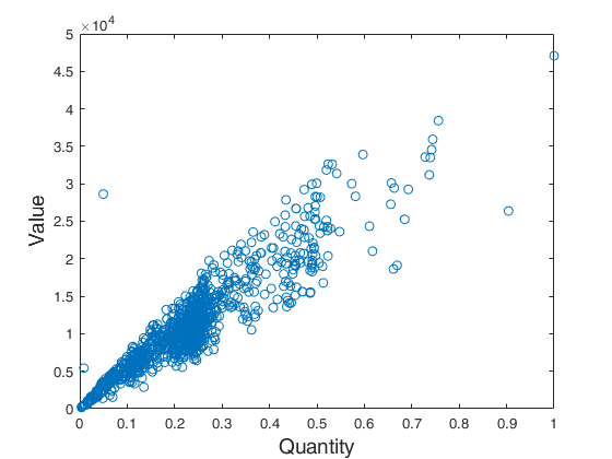
FSRH with all default options.Before running FSRH, data are plotted. Common part to all examples: load tradeH dataset.
XX=load('tradeH.txt');
y=XX(:,2);
X=XX(:,1);
X=X./max(X);
Z=log(X);
plot(X,y,'o')
fs=14;
ylabel('Value','FontSize',fs)
xlabel('Quantity','FontSize',fs)
out=FSRH(y,X,Z);
Total estimated time to complete LMS: 0.03 seconds
Warning: interchange greater than 10 when m=12
Number of units which entered=13
Warning: interchange greater than 10 when m=315
Number of units which entered=17
Warning: interchange greater than 10 when m=322
Number of units which entered=20
Warning: interchange greater than 10 when m=330
Number of units which entered=25
Warning: interchange greater than 10 when m=354
Number of units which entered=17
Warning: interchange greater than 10 when m=499
Number of units which entered=21
Warning: interchange greater than 10 when m=502
Number of units which entered=13
Warning: interchange greater than 10 when m=507
Number of units which entered=19
Warning: interchange greater than 10 when m=509
Number of units which entered=11
-------------------------
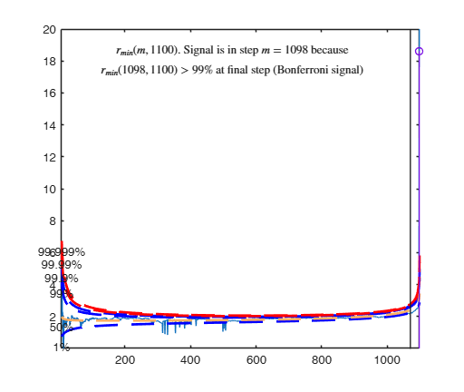
Signal detection loop
Signal is in penultimate step of the search
rmin(1098,1100)>99.9%
rmin(1098,1100)>99% at final step: Bonferroni signal in the final part of the search.
-------------------
Signal validation exceedance of upper envelopes
Validated signal
Warning: Upper limit of y axis of the mdr forward plot set to 20
-------------------------------
Start resuperimposing envelopes from step m=1097
Superimposition stopped because r_{min}(1098,1099)>99% envelope
$r_{min}(1098,1099)>99$\% envelope
----------------------------
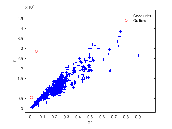
Final output
Number of units declared as outliers=2
Summary of the exceedances
1 99 999 9999 99999
88 3 2 2 2
FSRH with optional arguments.
Specifying the search initialization and controlling the y scale in plot.
XX=load('tradeH.txt');
y=XX(:,2);
X=XX(:,1);
X=X./max(X);
Z=log(X);
out=FSRH(y,X,Z,'init',round(length(y)/2),'plots',1,'ylim',[1.6 3]);
Input Arguments
y — Response variable.
Vector.
Response variable, specified as a vector of length n, where n is the number of observations. Each entry in y is the response for the corresponding row of X.
Missing values (NaN's) and infinite values (Inf's) are allowed, since observations (rows) with missing or infinite values will automatically be excluded from the computations.
Data Types: single| double
X — Predictor variables in the regression equation.
Matrix.
Matrix of explanatory variables (also called 'regressors') of dimension n x (p-1) where p denotes the number of explanatory variables including the intercept.
Rows of X represent observations, and columns represent variables. By default, there is a constant term in the model, unless you explicitly remove it using input option intercept, so do not include a column of 1s in X. Missing values (NaN's) and infinite values (Inf's) are allowed, since observations (rows) with missing or infinite values will automatically be excluded from the computations.
Data Types: single| double
Z — Predictor variables in the scedastic equation.
Matrix.
n x r matrix or vector of length r.
If Z is a n x r matrix it contains the r variables which form the scedastic function as follows (if input option art==1)
If Z is a vector of length r it contains the indexes of the columns of matrix X which form the scedastic function as follows \omega_i = 1 + exp(\gamma_0 + \gamma_1 X(i,Z(1)) + ...+ \gamma_{r} X(i,Z(r))) Therefore, if, for example, the explanatory variables responsible for heteroscedasticity are columns 3 and 5 of matrix X, it is possible to use both the syntax: FSRH(y,X,X(:,[3 5])) or the syntax: FSRH(y,X,[3 5])
Data Types: single| double
Name-Value Pair Arguments
Specify optional comma-separated pairs of Name,Value arguments.
Name is the argument name and Value
is the corresponding value. Name must appear
inside single quotes (' ').
You can specify several name and value pair arguments in any order as
Name1,Value1,...,NameN,ValueN.
 'intercept',false
, 'typeH','har'
, 'h',round(n*0,75)
, 'nsamp',1000
, 'lms',1
, 'plots',1
, 'init',100 starts monitoring from step m=100
, 'tag',{'plmdr' 'plyXplot'};
, 'gridsearch',1
, 'nocheck',true
, 'bivarfit',2
, 'multivarfit','1'
, 'labeladd','1'
, 'nameX',{'NameVar1','NameVar2'}
, 'namey','NameOfResponse'
, 'bonflev',0.99
, 'msg',1
, 'bsbmfullrank',1
intercept
—Indicator for constant term.true (default) | false.
Indicator for the constant term (intercept) in the fit, specified as the comma-separated pair consisting of 'Intercept' and either true to include or false to remove the constant term from the model.
Example: 'intercept',false
Data Types: boolean
typeH
—Parametric function to be used in the skedastic equation.character | String.
If typeH is 'art' (default) than the skedastic function is modelled as follows \sigma^2_i = \sigma^2 (1 + \exp(\gamma_0 + \gamma_1 Z(i,1) + \cdots + \gamma_{r} Z(i,r))) on the other hand, if typeH is 'har' then traditional formulation due to Harvey is used as follows \sigma^2_i = \exp(\gamma_0 + \gamma_1 Z(i,1) + \cdots + \gamma_{r} Z(i,r)) =\sigma^2 (\exp(\gamma_1 Z(i,1) + \cdots + \gamma_{r} Z(i,r))
Example: 'typeH','har'
Data Types: character or string
h
—The number of observations that have determined the least
trimmed squares estimator.scalar.
h is an integer greater or equal than p but smaller then n. Generally, if the purpose is outlier detection h=[0.5*(n+p+1)] (default value). h can be smaller than this threshold if the purpose is to find subgroups of homogeneous observations.
Example: 'h',round(n*0,75)
Data Types: double
nsamp
—Number of subsamples which will be extracted to find the
robust estimator.scalar.
If nsamp=0 all subsets will be extracted.
They will be (n choose p).
Remark: if the number of all possible subset is <1000, the default is to extract all subsets otherwise just 1000.
Example: 'nsamp',1000
Data Types: double
lms
—Criterion to use to find the initial
subset to initialize the search.scalar, vector | structure.
lms specifies the criterion to use to find the initial subset to initialize the search (LMS, LTS with concentration steps, LTS without concentration steps or subset supplied directly by the user).
The default value is 1 (Least Median of Squares is computed to initialize the search). On the other hand, if the user wants to initialize the search with LTS with all the default options for concentration steps then lms=2. If the user wants to use LTS without concentration steps, lms can be a scalar different from 1 or 2. If lms is a struct, it is possible to control a series of options for concentration steps (for more details see option lms inside LXS.m) LXS.
If, on the other hand, the user wants to initialize the search with a prespecified set of units there are two possibilities: 1) lms can be a vector with length greater than 1 which contains the list of units forming the initial subset. For example, if the user wants to initialize the search with units 4, 6 and 10 then lms=[4 6 10].
2) lms is a struct which contains a field named bsb which contains the list of units to initialize the search. For example, in the case of simple regression through the origin with just one explanatory variable, if the user wants to initialize the search with unit 3 then lms=struct;
| Value | Description |
|---|---|
bsb |
3. |
Example: 'lms',1
Data Types: double
plots
—Plot on the screen.scalar.
If plots=1 (default) the plot of minimum deletion residual with envelopes based on n observations and the scatterplot matrix with the outliers highlighted is produced.
If plots=2 the user can also monitor the intermediate plots based on envelope superimposition.
else no plot is produced.
Example: 'plots',1
Data Types: double
init
—Search initialization.scalar.
It specifies the initial subset size to start monitoring exceedances of minimum deletion residual, if init is not specified it set equal to: p+1, if the sample size is smaller than 40;
min(3*p+1,floor(0.5*(n+p+1))), otherwise.
Example: 'init',100 starts monitoring from step m=100
Data Types: double
tag
—tags to the plots which are created.character | cell array of characters.
This option enables to add a tag to the plots which are created. The default tag names are: fsr_mdrplot for the plot of mdr based on all the observations;
fsr_yXplot for the plot of y against each column of X with the outliers highlighted;
fsr_resuperplot for the plot of resuperimposed envelopes. The first plot with 4 panel of resuperimposed envelopes has tag fsr_resuperplot1, the second fsr_resuperplot2 ...
If tag is character or a cell of characters of length 1, it is possible to specify the tag for the plot of mdr based on all the observations;
If tag is a cell of length 2, it is possible to control both the tag for the plot of mdr based on all the observations and the tag for the yXplot with outliers highlighted.
If tag is a cell of length 3, the third element specifies the names of the plots of resuperimposed envelopes.
Example: 'tag',{'plmdr' 'plyXplot'};
Data Types: char or cell
gridsearch
—Algorithm to be used.scalar.
If gridsearch ==1 grid search will be used else (default) the scoring algorithm will be used.
Example: 'gridsearch',1
Data Types: double
nocheck
—Check input arguments.boolean.
If nocheck is equal to true, no check is performed on matrix y and matrix X. Notice that y and X are left unchanged. In other words, the additional column of ones for the intercept is not added. As default nocheck=false.
Example: 'nocheck',true
Data Types: boolean
bivarfit
—Superimpose bivariate least square lines.character.
This option adds one or more least square lines, based on SIMPLE REGRESSION of y on Xi, to the plots of y|Xi.
bivarfit = '' is the default: no line is fitted.
bivarfit = '1' fits a single ols line to all points of each bivariate plot in the scatter matrix y|X.
bivarfit = '2' fits two ols lines: one to all points and another to the group of the genuine observations. The group of the potential outliers is not fitted.
bivarfit = '0' fits one ols line to each group. This is useful for the purpose of fitting mixtures of regression lines.
bivarfit = 'i1' or 'i2' or 'i3' etc.
fits an ols line to a specific group, the one with index 'i' equal to 1, 2, 3 etc. Again, useful in case of mixtures.
Example: 'bivarfit',2
Data Types: char
multivarfit
—Superimpose multivariate least square lines.character.
This option adds one or more least square lines, based on MULTIVARIATE REGRESSION of y on X, to the plots of y|Xi.
multivarfit = '' is the default: no line is fitted.
multivarfit = '1' fits a single ols line to all points of each bivariate plot in the scatter matrix y|X. The line added to the scatter plot y|Xi is avconst + Ci*Xi, where Ci is the coefficient of Xi in the multivariate regression and avconst is the effect of all the other explanatory variables different from Xi evaluated at their centroid (that is overline{y}'C)) multivarfit = '2' equal to multivarfit ='1' but this time we also add the line based on the group of unselected observations (i.e. the normal units).
Example: 'multivarfit','1'
Data Types: char
labeladd
—Add outlier labels in plot.character.
If this option is '1', we label the outliers with the unit row index in matrices X and y. The default value is labeladd='', i.e. no label is added.
Example: 'labeladd','1'
Data Types: char
nameX
—Add variable labels in plot.cell array of strings.
labels of the variables of the regression dataset. If it is empty (default) the sequence X1, ..., Xp will be created automatically
Example: 'nameX',{'NameVar1','NameVar2'}
Data Types: cell
namey
—Add response label.character.
label of the response
Example: 'namey','NameOfResponse'
Data Types: char
ylim
—Control y scale in plot.vector.
minimum and maximum on the y axis. Default value is '' (automatic scale)
Example: 'ylim','[0,10]' sets the minim value to 0 and the
max to 10 on the y axis
Data Types: double
xlim
—Control x scale in plot.vector.
minimum and maximum on the x axis. Default value is '' (automatic scale)
Example: 'xlim','[0,10]' sets the minimum value to 0 and the
max to 10 on the x axis
Data Types: double
bonflev
—Signal to use to identify outliers.scalar.
option to be used if the distribution of the data is strongly non normal and, thus, the general signal detection rule based on consecutive exceedances cannot be used. In this case bonflev can be: - a scalar smaller than 1, which specifies the confidence level for a signal and a stopping rule based on the comparison of the minimum MD with a Bonferroni bound. For example, if bonflev=0.99 the procedure stops when the trajectory exceeds for the first time the 99% bonferroni bound.
- A scalar value greater than 1. In this case the procedure stops when the residual trajectory exceeds for the first time this value.
Default value is '', which means to rely on general rules based on consecutive exceedances.
Example: 'bonflev',0.99
Data Types: double
msg
—Level of output to display.scalar.
It controls whether to display or not messages on the screen If msg==1 (default) messages are displayed on the screen about step in which signal took place else no message is displayed on the screen
Example: 'msg',1
Data Types: double
bsbmfullrank
—Dealing with singular X matrix.scalar.
It tells how to behave in case subset at step m (say bsbm) produces a non singular X. In other words, this options controls what to do when rank(X(bsbm,:)) is smaller than number of explanatory variables. If bsbmfullrank =1 (default), these units (whose number is say mnofullrank) are constrained to enter the search in the final n-mnofullrank steps, else the search continues using as estimate of beta at step m, the estimate of beta found in the previous step.
Example: 'bsbmfullrank',1
Data Types: double
Output Arguments
out — description
Structure
T consists of a structure 'out' containing the following fields:
| Value | Description |
|---|---|
ListOut |
k x 1 vector containing the list of the units declared as outliers or empty if the sample is homogeneous. This field in future releases will be deleted because it will be replaced by out.outliers. |
outliers |
k x 1 vector containing the list of the units declared as outliers or empty if the sample is homogeneous. |
beta |
p-by-1 vector containing the estimated regression parameters (in step n-k). |
hetero |
r-by-1 vector containing the estimated parameters of the scedastic parameters (in step n-k) |
scale |
scalar containing the estimate of the scale (sigma). |
mdr |
(n-init) x 2 matrix: 1st col = fwd search index; 2nd col = value of minimum deletion residual in each step of the fwd search. |
Un |
(n-init) x 11 Matrix which contains the unit(s) included in the subset at each step of the fwd search. REMARK: in every step the new subset is compared with the old subset. Un contains the unit(s) present in the new subset but not in the old one. Un(1,2), for example, contains the unit included in step init+1. Un(end,2) contains the units included in the final step of the search. |
nout |
2 x 5 matrix containing the number of times mdr went out of particular quantiles. First row contains quantiles 1 99 99.9 99.99 99.999. Second row contains the frequency distribution. |
constr |
This output is produced only if the search found at a certain step is a non singular matrix X. In this case, the search run in a constrained mode, that is including the units which produced a singular matrix in the last n-constr steps. out.constr is a vector which contains the list of units which produced a singular X matrix |
class |
'FSRH'. |
References
Atkinson, A.C., Riani, M. and Torti, F. (2016), Robust methods for heteroskedastic regression, "Computational Statistics and Data Analysis", Vol. 104, pp. 209-222, http://dx.doi.org/10.1016/j.csda.2016.07.002 [ART]