FSRHbsb
FSRHbsb returns the units belonging to the subset in each step of the heteroskedastic forward search
Syntax
Description
Examples
FSRHbsb with all default options.
Common part to all examples: load tradeH dataset (used in the paper ART).
XX=load('tradeH.txt');
y=XX(:,2);
X=XX(:,1);
X=X./max(X);
Z=log(X);
Un=FSRHbsb(y,X,Z,[1:10]);
 FSRHbsb with optional arguments.
FSRHbsb with optional arguments.Suppress all messages about interchange with option msg.
% Common part to all examples: load tradeH dataset (used in the paper ART).
XX=load('tradeH.txt');
y=XX(:,2);
X=XX(:,1);
X=X./max(X);
Z=log(X);
Un=FSRHbsb(y,X,Z,[1:10],'plots',1,'msg',0);
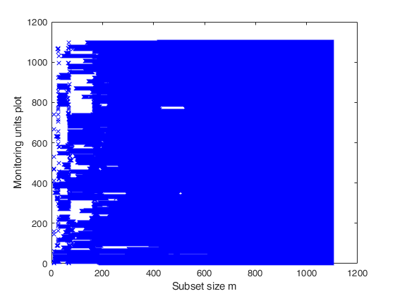
Monitoring the units belonging to subset in each step.
Common part to all examples: load tradeH dataset (used in the paper ART).
XX=load('tradeH.txt');
y=XX(:,2);
X=XX(:,1);
X=X./max(X);
Z=log(X);
[~,Un,BB]=FSRHmdr(y,X,Z,[1:10]);
[Unchk,BBchk]=FSRHbsb(y,X,Z,[1:10]);
% Test for equality BB and BBchk
disp(isequaln(BB,BBchk))
% Test for equality Un and Unchk
disp(isequaln(Un,Unchk))
Input Arguments
y — Response variable.
Vector.
Response variable, specified as a vector of length n, where n is the number of observations. Each entry in y is the response for the corresponding row of X.
Missing values (NaN's) and infinite values (Inf's) are allowed, since observations (rows) with missing or infinite values will automatically be excluded from the computations.
Data Types: single| double
X — Predictor variables in the regression equation.
Matrix.
Matrix of explanatory variables (also called 'regressors') of dimension n x (p-1) where p denotes the number of explanatory variables including the intercept.
Rows of X represent observations, and columns represent variables. By default, there is a constant term in the model, unless you explicitly remove it using input option intercept, so do not include a column of 1s in X. Missing values (NaN's) and infinite values (Inf's) are allowed, since observations (rows) with missing or infinite values will automatically be excluded from the computations.
Data Types: single| double
Z — Predictor variables in the scedastic equation.
Matrix.
n x r matrix or vector of length r.
If Z is a n x r matrix it contains the r variables which form the scedastic function as follows (if input option art==1)
If Z is a vector of length r it contains the indexes of the columns of matrix X which form the scedastic function as follows \omega_i = 1 + exp(\gamma_0 + \gamma_1 X(i,Z(1)) + ...+ \gamma_{r} X(i,Z(r))) Therefore, if, for example, the explanatory variables responsible for heteroscedasticity are columns 3 and 5 of matrix X, it is possible to use both the syntax: FSRHbsb(y,X,X(:,[3 5]),0) or the syntax: FSRHbsb(y,X,[3 5],0)
Data Types: single| double
bsb — list of units forming the initial subset.
Vector | 0.
If bsb=0 then the procedure starts with p units randomly chosen else if bsb is not 0 the search will start with m0=length(bsb)
Data Types: single| double
Name-Value Pair Arguments
Specify optional comma-separated pairs of Name,Value arguments.
Name is the argument name and Value
is the corresponding value. Name must appear
inside single quotes (' ').
You can specify several name and value pair arguments in any order as
Name1,Value1,...,NameN,ValueN.
 'init',100 starts monitoring from step m=100
, 'intercept',false
, 'typeH','har'
, 'nocheck',true
, 'msg',1
, 'gridsearch',0
, 'constr',[1 6 3]
, 'plots',1
init
—Search initialization.scalar.
It specifies the point where to start monitoring required diagnostics. If it is not specified it is set equal to: p+1, if the sample size is smaller than 40;
min(3*p+1,floor(0.5*(n+p+1))), otherwise.
The minimum value of init is 0. In this case, in the first step, we just use prior information.
Example: 'init',100 starts monitoring from step m=100
Data Types: double
intercept
—Indicator for constant term.true (default) | false.
Indicator for the constant term (intercept) in the fit, specified as the comma-separated pair consisting of 'Intercept' and either true to include or false to remove the constant term from the model.
Example: 'intercept',false
Data Types: boolean
typeH
—Parametric function to be used in the skedastic equation.string.
If typeH is 'art' (default) than the skedastic function is modelled as follows \sigma^2_i = \sigma^2 (1 + \exp(\gamma_0 + \gamma_1 Z(i,1) + \cdots + \gamma_{r} Z(i,r))) on the other hand, if typeH is 'har' then traditional formulation due to Harvey is used as follows \sigma^2_i = \exp(\gamma_0 + \gamma_1 Z(i,1) + \cdots + \gamma_{r} Z(i,r)) =\sigma^2 (\exp(\gamma_1 Z(i,1) + \cdots + \gamma_{r} Z(i,r))
Example: 'typeH','har'
Data Types: string
nocheck
—Check input arguments.boolean.
If nocheck is equal to true, no check is performed on matrix y and matrix X. Notice that y and X are left unchanged. In other words, the additional column of ones for the intercept is not added. As default nocheck=false.
Example: 'nocheck',true
Data Types: boolean
msg
—Level of output to display.scalar.
It controls whether to display or not messages about great interchange on the screen If msg==1 (default) messages are displayed on the screen, else no message is displayed on the screen
Example: 'msg',1
Data Types: double
gridsearch
—Algorithm to be used.scalar.
If gridsearch ==1 grid search will be used, else the scoring algorithm will be used.
REMARK: the grid search has only been implemented when there is just one explanatory variable which controls heteroskedasticity.
Example: 'gridsearch',0
Data Types: double
constr
—units which are forced to join the search in the last r steps.vector.
r x 1 vector. The default is constr=''. No constraint is imposed
Example: 'constr',[1 6 3]
Data Types: double
bsbsteps
—Save the units forming subsets in selected steps.vector.
It specifies for which steps of the fwd search it is necessary to save the units forming subset. If bsbsteps is 0, we store the units forming subset in all steps. The default is: store the units forming subset in all steps if n<=5000, else to store the units forming subset at steps init and steps which are multiple of 100. For example, as default, if n=7530 and init=6, units forming subset are stored for m=init, 100, 200, ..., 7500.
Example: 'bsbsteps',[100 200] stores the unis forming
subset in steps 100 and 200.
Data Types: double
plots
—Plot on the screen.scalar.
If plots=1 the monitoring units plot is displayed on the screen. The default value of plots is 0 (that is no plot is produced on the screen).
Example: 'plots',1
Data Types: double
Output Arguments
Un —Units included in each step.
Matrix
(n-init) x 11 Matrix which contains the unit(s) included in the subset at each step of the search.
REMARK: in every step the new subset is compared with the old subset. Un contains the unit(s) present in the new subset but not in the old one.
Un(1,2), for example, contains the unit included in step init+1.
Un(end,2) contains the units included in the final step of the search.
BB —Units belonging to subset in each step.
Matrix
n x (n-init+1) matrix which contains the units belonging to the subset at each step of the forward search.
1st col = index forming subset in the initial step ...
last column = units forming subset in the final step (i.e. all units).
References
Atkinson, A.C., Riani, M. and Torti, F. (2016), Robust methods for heteroskedastic regression, "Computational Statistics and Data Analysis", Vol. 104, pp. 209-222, http://dx.doi.org/10.1016/j.csda.2016.07.002 [ART]