FSRBbsb

FSRBbsb returns the units belonging to the subset in each step of the Bayesian forward search

Syntax

  • Un=FSRBbsb(y, X, beta0, R, tau0, n0)example
  • Un=FSRBbsb(y, X, beta0, R, tau0, n0,Name,Value)example
  • [Un,BB]=FSRBbsb(___)example

Description

example

Un =FSRBbsb(y, X, beta0, R, tau0, n0) FSRBbsb with all default options.

example

Un =FSRBbsb(y, X, beta0, R, tau0, n0, Name, Value) FSRBbsb with optional arguments.

example

[Un, BB] =FSRBbsb(___) Compare units belonging to subsets.

Examples

expand all

  • FSRBbsb with all default options.
  • Common part to all examples: load Houses Price Dataset.

    load hprice.txt;
    % setup parameters
    n=size(hprice,1);
    y=hprice(:,1);
    X=hprice(:,2:5);
    n0=5;
    % set \beta components
    beta0=0*ones(5,1);
    beta0(2,1)=10;
    beta0(3,1)=5000;
    beta0(4,1)=10000;
    beta0(5,1)=10000;
    % $\tau$
    s02=1/4.0e-8;
    tau0=1/s02;
    % R prior settings
    R=2.4*eye(5);
    R(2,2)=6e-7;
    R(3,3)=.15;
    R(4,4)=.6;
    R(5,5)=.6;
    R=inv(R);
    Unchk=FSRBbsb(y,X,beta0, R, tau0, n0);

  • FSRBbsb with optional arguments.
  • Display the monitoring units plot. Suppress all messages about interchange with option msg.

    load hprice.txt;
    % setup parameters
    n=size(hprice,1);
    y=hprice(:,1);
    X=hprice(:,2:5);
    n0=5;
    % set \beta components
    beta0=0*ones(5,1);
    beta0(2,1)=10;
    beta0(3,1)=5000;
    beta0(4,1)=10000;
    beta0(5,1)=10000;
    % $\tau$
    s02=1/4.0e-8;
    tau0=1/s02;
    % R prior settings
    R=2.4*eye(5);
    R(2,2)=6e-7;
    R(3,3)=.15;
    R(4,4)=.6;
    R(5,5)=.6;
    R=inv(R);
    [~,Un,BB]=FSRBmdr(y,X,beta0, R, tau0, n0);
    [Unchk,BBchk]=FSRBbsb(y,X,beta0,R,tau0,n0,'plots',1,'msg',0);
    Click here for the graphical output of this example (link to Ro.S.A. website).

  • Compare units belonging to subsets.
  • Test procedures FSRBmdr and FSRBbsb to find out whether they produce the same results in terms of units belonging to subset

    load hprice.txt;
    % setup parameters
    n=size(hprice,1);
    y=hprice(:,1);
    X=hprice(:,2:5);
    n0=5;
    % set \beta components
    beta0=0*ones(5,1);
    beta0(2,1)=10;
    beta0(3,1)=5000;
    beta0(4,1)=10000;
    beta0(5,1)=10000;
    % $\tau$
    s02=1/4.0e-8;
    tau0=1/s02;
    % R prior settings
    R=2.4*eye(5);
    R(2,2)=6e-7;
    R(3,3)=.15;
    R(4,4)=.6;
    R(5,5)=.6;
    R=inv(R);
    [~,Un,BB]=FSRBmdr(y,X,beta0, R, tau0, n0);
    [Unchk,BBchk]=FSRBbsb(y,X,beta0, R, tau0, n0);
    % Test for equality BB and BBchk
    disp(isequaln(BB,BBchk))
    % Test for equality Un and Unchk
    disp(isequaln(Un,Unchk))

    Input Arguments

    expand all

    y — Response variable. Vector.

    A vector with n elements that contains the response variable.

    Missing values (NaN's) and infinite values (Inf's) are allowed, since observations (rows) with missing or infinite values will automatically be excluded from the computations.

    Data Types: single| double

    X — Predictor variables. Matrix.

    Data matrix of explanatory variables (also called 'regressors') of dimension (n x p-1).

    Rows of X represent observations, and columns represent variables. Missing values (NaN's) and infinite values (Inf's) are allowed, since observations (rows) with missing or infinite values will automatically be excluded from the computations.

    PRIOR INFORMATION $\beta$ is assumed to have a normal distribution with mean $\beta_0$ and (conditional on $\tau_0$) covariance $(1/\tau_0) (X_0'X_0)^{-1}$.

    $\beta \sim N( \beta_0, (1/\tau_0) (X_0'X_0)^{-1} )$

    Data Types: single| double

    beta0 — Prior mean of $\beta$. p-times-1 vector.

    Data Types: single| double

    R — Matrix associated with covariance matrix of $\beta$. p-times-p positive definite matrix.

    It can be interpreted as $X_0'X_0$ where $X_0$ is a n0 x p matrix coming from previous experiments (assuming that the intercept is included in the model) The prior distribution of $\tau_0$ is a gamma distribution with parameters $a_0$ and $b_0$, that is \[ p(\tau_0) \propto \tau^{a_0-1} \exp (-b_0 \tau) \qquad E(\tau_0)= a_0/b_0 \]

    Data Types: single| double

    tau0 — Prior estimate of tau. Scalar.

    Prior estimate of $\tau=1/ \sigma^2 =a_0/b_0$.

    Data Types: single| double

    n0 — Number of previous experiments. Scalar.

    Sometimes it helps to think of the prior information as coming from n0 previous experiments. Therefore we assume that matrix X0 (which defines R), was made up of n0 observations.

    Data Types: single| double

    Name-Value Pair Arguments

    Specify optional comma-separated pairs of Name,Value arguments. Name is the argument name and Value is the corresponding value. Name must appear inside single quotes (' '). You can specify several name and value pair arguments in any order as Name1,Value1,...,NameN,ValueN.

    Example: 'bsb',[3,6,9] , 'init',100 starts monitoring from step m=100 , 'intercept',false , 'plots',1 , 'bsbsteps',[10,20,30] , 'nocheck',true , 'msg',1

    bsb —units forming initial subset.vector.

    m x 1 vector containing the units forming initial subset. The default value of bsb is '' (empty value), that is we initialize the search just using prior information.

    Example: 'bsb',[3,6,9]

    Data Types: double

    init —Search initialization.scalar.

    It specifies the point where to start monitoring required diagnostics. If it is not specified it is set equal to: p+1, if the sample size is smaller than 40;

    min(3*p+1,floor(0.5*(n+p+1))), otherwise.

    The minimum value of init is 0. In this case in the first step we start monitoring at step m=0 (step just based on prior information)

    Example: 'init',100 starts monitoring from step m=100

    Data Types: double

    intercept —Indicator for constant term.true (default) | false.

    Indicator for the constant term (intercept) in the fit, specified as the comma-separated pair consisting of 'Intercept' and either true to include or false to remove the constant term from the model.

    Example: 'intercept',false

    Data Types: boolean

    plots —Plot on the screen.scalar.

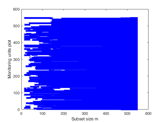
    If plots=1 the monitoring units plot is displayed on the screen. The default value of plots is 0 (that is no plot is produced on the screen).

    Example: 'plots',1

    Data Types: double

    bsbsteps —steps of the fwd search where to save the units forming subset.vector.

    If bsbsteps is 0 we store the units forming subset in all steps. The default is store the units forming subset in all steps if n<5000, else to store the units forming subset at steps init and steps which are multiple of 100. For example, if n=753 and init=6, units forming subset are stored for m=init, 100, 200, 300, 400, 500 and 600.

    Example: 'bsbsteps',[10,20,30]

    Data Types: double

    nocheck —Check input arguments.boolean.

    If nocheck is equal to true no check is performed on matrix y and matrix X. Notice that y and X are left unchanged. In other words the additional column of ones for the intercept is not added. As default nocheck=false.

    Example: 'nocheck',true

    Data Types: boolean

    msg —Level of output to display.scalar.

    It controls whether to display or not messages about great interchange on the screen If msg==1 (default) messages are displayed on the screen else no message is displayed on the screen

    Example: 'msg',1

    Data Types: double

    Output Arguments

    expand all

    Un —Units included in each step. Matrix

    (n-init) x 11 Matrix which contains the unit(s) included in the subset at each step of the search.

    REMARK: in every step the new subset is compared with the old subset. Un contains the unit(s) present in the new subset but not in the old one.

    Un(1,2) for example contains the unit included in step init+1.

    Un(end,2) contains the units included in the final step of the search.

    BB —Units belonging to subset in each step. Matrix

    n x (n-init+1) matrix which contains the units belonging to the subset at each step of the forward search.

    1st col = index forming subset in the initial step ...

    last column = units forming subset in the final step (i.e. all units).

    References

    Chaloner, K. and Brant, R. (1988), A Bayesian Approach to Outlier Detection and Residual Analysis, "Biometrika", Vol. 75, pp. 651-659.

    Riani, M., Corbellini, A. and Atkinson, A.C. (2018), Very Robust Bayesian Regression for Fraud Detection, "International Statistical Review", http://dx.doi.org/10.1111/insr.12247

    Atkinson, A.C., Corbellini, A. and Riani, M., (2017), Robust Bayesian Regression with the Forward Search: Theory and Data Analysis, "Test", Vol. 26, pp. 869-886, https://doi.org/10.1007/s11749-017-0542-6

    See Also

    |

    This page has been automatically generated by our routine publishFS