boxplotb

boxplotb computes a bivariate boxplot

Syntax

Description

example

out =boxplotb(Y) boxplotb with all default options.

example

out =boxplotb(Y, Name, Value) boxplotb with optional arguments.

Examples

expand all

  • boxplotb with all default options.
  • Bivariate boxplot of the writing data at time t=5.

    % This example reproduces Figure 1 of Corbellini, Riani and Atkinson,
    % 2015, Statistical Methods and Applications
    close all
    X=load('writingdata.txt');
    out=boxplotb(X);
    xlabel('horizontal coordinate')
    ylabel('vertical coordinate')
    title('Bivariate boxplot of the writing data at time $t=5$','Interpreter','Latex')
    Click here for the graphical output of this example (link to Ro.S.A. website).

  • boxplotb with optional arguments.
  • Bivariate boxplot of the stars data This example reproduces Figure 4 of Zani Riani and Corbellini

    close all
    X=load('stars.txt');
    out=boxplotb(X,'strictlyinside',1);
    xlabel('Log effective surface temperature')
    ylabel('Log light intensity')
    Click here for the graphical output of this example (link to Ro.S.A. website).

    Related Examples

    expand all

  • Bivariate boxplot of the brain data.
  • This example reproduces Figure 4 of Zani Riani and Corbellini

    close all
    X=load('bodybrain.txt');
    X=log10(X);
    out=boxplotb(X);
    xlabel('Log (to the base 10) body weight')
    ylabel('Log (to the base 10) brain weight')
    title('Bivariate boxplot of Log brain weight and Log body weight for 28 animals')

  • Bivariate boxplot of the stars data.
  • Now we change the colors of the inner and outer contour to white In this example we explore the various graphical options

    close all
    X=load('stars.txt');
    plots=struct;
    plots.InnerColor=[0 0 0]+1; % remove the color for the hinge
    plots.OuterColor=[0 0 0]+1; % remove the color for the fence
    plots.labeladd=0; % do not include the labels for the outliers
    plots.xlim=[min(X(:,1)) max(X(:,1))];  % tight xlim
    plots.ylim=[min(X(:,2)) max(X(:,2))];  % tight ylim
    out=boxplotb(X,'strictlyinside',1,'plots',plots);
    xlabel('Log effective surface temperature')
    ylabel('Log light intensity')

  • Bivariate boxplot of two variables of Emilia Romagna data.
  • This example reproduces Figure 2 of Zani Riani and Corbellini

    close all
    load('emilia2001')
    Y=emilia2001{:,:};
    % Extract the variables y1 and y3
    % y1= Percentage of infant population (that is the percentage of
    % population aged less than 10)
    % y3 = % of single member (one component) families
    X=Y(:,[1 3]);
    % In order to reproduce exactly Figure 2 of Zani, Riani and Corbellini
    % (1998), CSDA, we remove municipalities with a percentage of single
    % members greater than 45%
    X=X(X(:,2)<45,:);
    out=boxplotb(X,'strictlyinside',1);
    xlabel('y1=Percentage of infant population')
    ylabel('y3 = Percentage of single member families')

    Input Arguments

    expand all

    Y — Observations. Matrix.

    n x 2 data matrix: n observations and 2 variables. Rows of Y represent observations, and columns represent variables.

    Data Types: single| double

    Name-Value Pair Arguments

    Specify optional comma-separated pairs of Name,Value arguments. Name is the argument name and Value is the corresponding value. Name must appear inside single quotes (' '). You can specify several name and value pair arguments in any order as Name1,Value1,...,NameN,ValueN.

    Example: 'coeff',1.68 , 'strictlyinside',1 , 'plots',1 , 'resolution',5000

    coeff —expansion factor.scalar.

    Coefficient which enables us to pass from a contour which contains 50% of the data (hinge) to a contour which contains a prespecified portion of the data.

    Table below (taken from Zani, Riani and Corbellini, 1998, CSDA) shows the coefficients which must be used to obtain a theoretical threshold of 75, 90, 95 or 99 per cent in presence of normally distributed data: confidence level 0.75 -> coefficient 0.43;

    confidence level 0.90 -> coefficient 0.83;

    confidence level 0.95 -> coefficient 1.13;

    confidence level 0.99 -> coefficient 1.68.

    Remark: The default value of coeff is 1.68, that is 99% confidence level contours are produced.

    Example: 'coeff',1.68

    Data Types: double

    strictlyinside —additional peeling.scalar.

    If strictlyinside=1 an additional convex hull is done on the 50% hull in order to increase the robustness properties of the method. In fact there may in general be some loss of robustness in small samples due to the use of peeling, therefore if we suspect to be in presence of a considerable propotion of outliers it may be necessary to do an additional peeling.

    The default value of strictlyinside is 0.

    Example: 'strictlyinside',1

    Data Types: double

    plots —graphical output.missing value | scalar | structure.

    This option specifies whether it is necessary to produce the bivariate boxplot on the screen.

    If plots is a missing value or is a scalar equal to 0 no plot is produced.

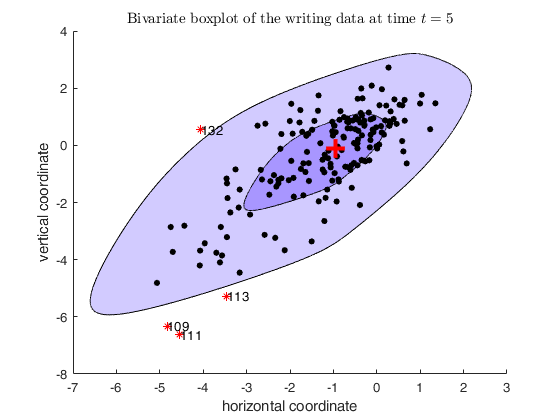
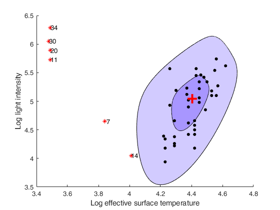
    If plots is a scalar equal to 1 (default) the bivariate boxplot with the outliers labelled is produced.

    If plots is a structure it may contain the following fields:

    Value Description
    ylim

    vector with two elements controlling minimum and maximum on the y axis. Default value is '' (automatic scale).

    xlim

    vector with two elements controlling minimum and maximum on the x axis. Default value is '' (automatic scale).

    labeladd

    if this option is '1', the outliers in the scatter plot are labelled with the unit row index. The default value is labeladd='1', i.e. the row numbers are added. plots.labeladd='' means no labelling.

    InnerColor

    a three element vector which specifies the color in RGB format to fill the inner contour (hinge). The default value of InnerColor is InnerColor=[168/255 150/255 255/255].

    OuterColor

    a three element vector which specifies the color in RGB format to fill the outer contour (fence). The default value of OuterColor is OuterColor=[210/255 203/255 255/255].

    Example: 'plots',1

    Data Types: [],double, struct

    resolution —resolution to use.scalar.

    Resolution which must be used to produce the inner and outer spline.

    The default value of resolution is 1000, that is the splines are plotted on the screen using 1000-by-(number of vertices of the inner hull) points.

    Example: 'resolution',5000

    Data Types: double

    Output Arguments

    expand all

    out — description Structure

    Structure which contains the following fields

    Value Description
    outliers

    vector containing the list of the units which lie outside the outer contour.

    REMARK: if no unit lies outside the outer spline outliers is a Empty matrix: 0-by-1

    cent

    2 x 1 vector containing the coordinates of the robust centroid.

    cent[1] = x coordinate;

    cent[2] = y coordinate.

    Spl

    r-by-4 matrix containing the coordinates of the inner and outer spline. r (rows of matrix Spl) is approximately equal to the number of vertices of the inner hull multiplied by the resolution which is used.

    The first two columns refer to the (x,y) coordinates of the inner spline.

    The last two columns refer to the (x,y) coordinates of the outer spline.

    handles

    r-by-1 matrix containing the handles of the contours and centroid. It can be used to control the display of these objects, for example using ClickableMultiLegend.

    References

    Zani, S., Riani M. and Cerioli A. (1998), Robust bivariate boxplots and multiple outlier detection, "Computational Statistics and Data Analysis", Vol. 28, pp. 257-270.

    Corbellini A., Riani M. and Atkinson A.C. (2015), Discussion of the paper 'Multivariate Functional Outlier Detection' by Hubert, Rousseeuw and Segaert, "Statistical Methods and Applications".

    See Also

    |

    This page has been automatically generated by our routine publishFS