CorAna
CorAna performs correspondence analysis
Description
Examples
 CorAna with name pairs.
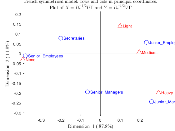
CorAna with name pairs.Input is the contingency table, labels for rows and columns are supplied.
% Data are read from the txt file
load('smoke.txt')
labels_rows= {'Senior-Managers' 'Junior-Managers' 'Senior-Employees' 'Junior-Employees' 'Secretaries'};
labels_columns= {'None' 'Light' 'Medium' 'Heavy'};
N=crosstab(smoke(:,1),smoke(:,2));
out=CorAna(N,'Lr',labels_rows,'Lc',labels_columns);
Summary
             Singular_value     Inertia      Accounted_for    Cumulative
             ______________    __________    _____________    __________

    dim_1        0.27342         0.074759        0.87756       0.87756
    dim_2        0.10009         0.010017        0.11759       0.99515
    dim_3       0.020337       0.00041357      0.0048547             1

ROW POINTS
Results for dimension: 1
                         Scores      CntrbPnt2In    CntrbDim2In
                        _________    ___________    ___________

    Senior_Managers     -0.065768     0.0032977      0.092232
    Junior_Managers       0.25896      0.083659        0.5264
    Senior_Employees     -0.38059       0.51201       0.99903
    Junior_Employees      0.23295       0.33097       0.94193
    Secretaries          -0.20109      0.070064       0.86535

Results for dimension: 2
                         Scores     CntrbPnt2In    CntrbDim2In
                        ________    ___________    ___________

    Senior_Managers     -0.19374       0.21356        0.80034
    Junior_Managers      -0.2433       0.55115        0.46468
    Senior_Employees    -0.01066     0.0029976     0.00078372
    Junior_Employees    0.057744       0.15177       0.057876
    Secretaries         0.078911      0.080522        0.13326

COLUMN POINTS
Results for dimension: 1
               Scores     CntrbPnt2In    CntrbDim2In
              ________    ___________    ___________

    None      -0.39331        0.654        0.99402
    Light     0.099456      0.03085        0.32673
    Medium     0.19632      0.16562        0.98185
    Heavy      0.29378      0.14954         0.6844

Results for dimension: 2
               Scores      CntrbPnt2In    CntrbDim2In
              _________    ___________    ___________

    None      -0.030492      0.029336      0.0059745
    Light       0.14106       0.46317        0.65729
    Medium    0.0073591     0.0017368      0.0013796
    Heavy      -0.19777       0.50575        0.31015

-----------------------------------------------------------
Overview ROW POINTS
                          Mass       Score_1     Score_2      Inertia     CntrbPnt2In_1    CntrbPnt2In_2    CntrbDim2In_1    CntrbDim2In_2
                        ________    _________    ________    _________    _____________    _____________    _____________    _____________

    Senior_Managers     0.056995    -0.065768    -0.19374    0.0026729      0.0032977          0.21356        0.092232           0.80034
    Junior_Managers     0.093264      0.25896     -0.2433     0.011881       0.083659          0.55115          0.5264           0.46468
    Senior_Employees     0.26425     -0.38059    -0.01066     0.038314        0.51201        0.0029976         0.99903        0.00078372
    Junior_Employees     0.45596      0.23295    0.057744     0.026269        0.33097          0.15177         0.94193          0.057876
    Secretaries          0.12953     -0.20109    0.078911     0.006053       0.070064         0.080522         0.86535           0.13326

Overview COLUMN POINTS
               Mass      Score_1      Score_2      Inertia     CntrbPnt2In_1    CntrbPnt2In_2    CntrbDim2In_1    CntrbDim2In_2
              _______    ________    _________    _________    _____________    _____________    _____________    _____________

    None      0.31606    -0.39331    -0.030492     0.049186         0.654          0.029336         0.99402         0.0059745
    Light     0.23316    0.099456      0.14106    0.0070588       0.03085           0.46317         0.32673           0.65729
    Medium    0.32124     0.19632    0.0073591      0.01261       0.16562         0.0017368         0.98185         0.0013796
    Heavy     0.12953     0.29378     -0.19777     0.016335       0.14954           0.50575          0.6844           0.31015

-----------------------------------------------------------
Legend
Row scores in principal coordinates
Column scores in principal coordinates
CntrbPnt2In = relative contribution of points to explain total Inertia of the latent dimension
              The sum of the numbers in a column is equal to 1
CntrbDim2In = relative contribution of latent dimension to explain total Inertia of a point
              CntrbDim2In_1+CntrbDim2In_2+...+CntrbDim2In_K=1

Related Examples
CorAna with supplementary rows and supplementary columns.
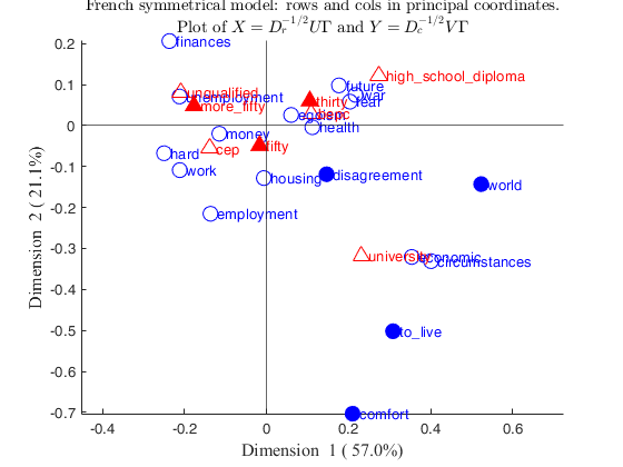
CorAna with supplementary rows and supplementary columns.Children data Active rows = 1:15 Active columns = 1:5
N=[51  64  32  29  17  59  66  70;
53  90  78  75  22  115  117  86;
71  111  50  40  11  79  88  177;
1  7  5  5  4  9  8  5;
7  11  4  3  2  2  17  18;
7  13  12  11  11  18  19  17;
21  37  14  26  9  14  34  61;
12  35  19  6  7  21  30  28;
10  7  7  3  1  8  12  8;
4  7  7  6  2  7  6  13;
8  22  7  10  5  10  27  17;
25  45  38  38  13  48  59  52;
18  27  20  19  9  13  29  53;
35  61  29  14  12  30  63  58;
2  4  3  1  4  nan  nan  nan    ;
2  8  2  5  2  nan  nan  nan;
1  5  4  6  3  nan  nan  nan;
3  3  1  3  4  nan  nan  nan];
% rowslab = cell containing row labels
rowslab={'money','future','unemployment','circumstances',...
'hard','economic','egoism','employment','finances',...
'war','housing','fear','health','work','comfort','disagreement',...
'world','to_live'};
% colslab = cell containing column labels
colslab={'unqualified','cep','bepc','high_school_diploma','university',...
'thirty','fifty','more_fifty'};
tableN=array2table(N,'VariableNames',colslab,'RowNames',rowslab);
% Extract just active rows and active columns
Nactive=tableN(1:14,1:5);
% Define tables containing supplementary rows and supplementary cols
Nsupr=tableN(15:18,1:5);
Nsupc=tableN(1:14,6:8);
Sup=struct;
Sup.r=Nsupr;
Sup.c=Nsupc;
out=CorAna(Nactive,'Sup',Sup);
Summary
             Singular_value     Inertia     Accounted_for    Cumulative
             ______________    _________    _____________    __________

    dim_1        0.18815        0.035402       0.57043        0.57043
    dim_2        0.11452        0.013115       0.21132        0.78175
    dim_3       0.085447       0.0073011       0.11764        0.89939
    dim_4       0.079018       0.0062439       0.10061              1

ROW POINTS
Results for dimension: 1
                      Scores      CntrbPnt2In    CntrbDim2In
                     _________    ___________    ___________

    money             -0.11527      0.045499        0.42845
    future             0.17645       0.17567        0.71562
    unemployment      -0.21223       0.22616        0.87492
    circumstances      0.40092      0.062745        0.58397
    hard              -0.24998      0.029938        0.88369
    economic           0.35396       0.12005        0.48362
    egoism            0.059889     0.0068096       0.073339
    employment        -0.13675      0.026215         0.1643
    finances            -0.237      0.027904        0.27623
    war                0.21682      0.021688        0.74907
    housing          -0.006681    4.1183e-05     0.00072894
    fear               0.20335       0.11666        0.90069
    health             0.11165      0.020571        0.79911
    work              -0.21168       0.12005        0.75402

Results for dimension: 2
                       Scores      CntrbPnt2In    CntrbDim2In
                     __________    ___________    ___________

    money             -0.020046     0.0037146       0.012958
    future             0.097863       0.14587        0.22013
    unemployment       0.070718      0.067786       0.097145
    circumstances      -0.33099       0.11544          0.398
    hard               -0.06765     0.0059184       0.064717
    economic           -0.32072       0.26604        0.39705
    egoism             0.025667     0.0033763       0.013471
    employment         -0.21539       0.17555         0.4076
    finances            0.20598      0.056902        0.20867
    war                0.074663     0.0069419       0.088821
    housing            -0.12824       0.04096        0.26858
    fear               0.058068      0.025678       0.073446
    health           -0.0042912    8.2025e-05      0.0011804
    work               -0.10888      0.085745        0.19951

COLUMN POINTS
Results for dimension: 1
                            Scores     CntrbPnt2In    CntrbDim2In
                           ________    ___________    ___________

    unqualified            -0.20932       0.2511        0.67619
    cep                    -0.13858      0.18297        0.64492
    bepc                    0.10876     0.067579         0.3119
    high_school_diploma     0.27404      0.37976        0.75817
    university              0.23123      0.11859        0.31171

Results for dimension: 2
                            Scores      CntrbPnt2In    CntrbDim2In
                           _________    ___________    ___________

    unqualified             0.080727      0.10082        0.10058
    cep                    -0.056047     0.080794        0.10549
    bepc                    0.028483     0.012512       0.021393
    high_school_diploma      0.12134      0.20099        0.14865
    university              -0.31786      0.60488          0.589

-----------------------------------------------------------
Overview ROW POINTS
                       Mass       Score_1      Score_2       Inertia      CntrbPnt2In_1    CntrbPnt2In_2    CntrbDim2In_1    CntrbDim2In_2
                     ________    _________    __________    __________    _____________    _____________    _____________    _____________

    money             0.12123     -0.11527     -0.020046     0.0037595       0.045499        0.0037146          0.42845         0.012958
    future            0.19975      0.17645      0.097863     0.0086904        0.17567          0.14587          0.71562          0.22013
    unemployment      0.17776     -0.21223      0.070718     0.0091512        0.22616         0.067786          0.87492         0.097145
    circumstances    0.013819      0.40092      -0.33099     0.0038038       0.062745          0.11544          0.58397            0.398
    hard              0.01696     -0.24998      -0.06765     0.0011994       0.029938        0.0059184          0.88369         0.064717
    economic          0.03392      0.35396      -0.32072     0.0087874        0.12005          0.26604          0.48362          0.39705
    egoism           0.067211     0.059889      0.025667     0.0032871      0.0068096        0.0033763         0.073339         0.013471
    employment       0.049623     -0.13675      -0.21539     0.0056484       0.026215          0.17555           0.1643           0.4076
    finances         0.017588       -0.237       0.20598     0.0035763       0.027904         0.056902          0.27623          0.20867
    war              0.016332      0.21682      0.074663      0.001025       0.021688        0.0069419          0.74907         0.088821
    housing          0.032663    -0.006681      -0.12824     0.0020001     4.1183e-05          0.04096       0.00072894          0.26858
    fear             0.099874      0.20335      0.058068     0.0045852        0.11666         0.025678          0.90069         0.073446
    health           0.058417      0.11165    -0.0042912    0.00091131       0.020571       8.2025e-05          0.79911        0.0011804
    work             0.094849     -0.21168      -0.10888     0.0056364        0.12005         0.085745          0.75402          0.19951

Overview COLUMN POINTS
                             Mass      Score_1      Score_2      Inertia     CntrbPnt2In_1    CntrbPnt2In_2    CntrbDim2In_1    CntrbDim2In_2
                           ________    ________    _________    _________    _____________    _____________    _____________    _____________

    unqualified             0.20289    -0.20932     0.080727     0.013146        0.2511          0.10082          0.67619          0.10058
    cep                     0.33731    -0.13858    -0.056047     0.010044       0.18297         0.080794          0.64492          0.10549
    bepc                    0.20226     0.10876     0.028483    0.0076704      0.067579         0.012512           0.3119         0.021393
    high_school_diploma     0.17902     0.27404      0.12134     0.017732       0.37976          0.20099          0.75817          0.14865
    university             0.078518     0.23123     -0.31786     0.013468       0.11859          0.60488          0.31171            0.589

-----------------------------------------------------------
Legend
Row scores in principal coordinates
Column scores in principal coordinates
CntrbPnt2In = relative contribution of points to explain total Inertia of the latent dimension
              The sum of the numbers in a column is equal to 1
CntrbDim2In = relative contribution of latent dimension to explain total Inertia of a point
              CntrbDim2In_1+CntrbDim2In_2+...+CntrbDim2In_K=1
Example of interpretation of values close to the center.
Example of interpretation of values close to the center.
N=[80  20  90  90  5  100  40
50  40  40  70  10  100  40
10  70  20  90  80  99  40
0  80  2  20  95  20  40
35  52  38  47  48  80  40];
rl=["Dog" "Cat" "Rat" "Cockroach" "Wallaby"];
cl=["Big" "Athletic" "Friendly"  "Trainable" "Resourceful" "Animal" "Lucky"];
Ntable=array2table(N,"RowNames",rl,"VariableNames",cl);
out=CorAna(Ntable);
% In the center of the map we have Wallaby and Lucky. Does this mean
% wallabies are lucky animals? No. Wallaby is pretty average on all the
% variables being measured. As it has nothing that differentiates it, the
% result is that it is in the middle of the map (i.e., near the origin).
% Similarly, Lucky does not differentiate, so it is also near the center.
% That they are both in the center tells us that they are both indistinct,
% and that is all that they have in common (in the data).
Summary
             Singular_value     Inertia     Accounted_for    Cumulative
             ______________    _________    _____________    __________

    dim_1        0.50576          0.2558        0.89448       0.89448
    dim_2        0.14914        0.022243       0.077779       0.97226
    dim_3       0.081626       0.0066627       0.023299       0.99556
    dim_4        0.03564       0.0012702      0.0044417             1

ROW POINTS
Results for dimension: 1
                  Scores     CntrbPnt2In    CntrbDim2In
                 ________    ___________    ___________

    Dog          -0.59431        0.3295       0.94186
    Cat           -0.3256      0.081449       0.81272
    Rat           0.27706      0.068913       0.57861
    Cockroach     0.95997       0.51987       0.96141
    Wallaby      0.019153    0.00027378      0.033895

Results for dimension: 2
                  Scores      CntrbPnt2In    CntrbDim2In
                 _________    ___________    ___________

    Dog           -0.12157      0.15856       0.039411
    Cat           0.079165     0.055371       0.048044
    Rat            0.22533      0.52422        0.38272
    Cockroach     -0.18988      0.23391       0.037614
    Wallaby      -0.057062     0.027946        0.30085

COLUMN POINTS
Results for dimension: 1
                    Scores     CntrbPnt2In    CntrbDim2In
                   ________    ___________    ___________

    Big            -0.68224       0.17879       0.90397
    Athletic        0.54545        0.1711       0.97126
    Friendly       -0.60693       0.15363       0.86806
    Trainable      -0.19488      0.026427       0.47685
    Resourceful     0.89767       0.42097       0.98264
    Animal          -0.2172      0.041317       0.59767
    Lucky           0.13298     0.0077629       0.55129

Results for dimension: 2
                    Scores      CntrbPnt2In    CntrbDim2In
                   _________    ___________    ___________

    Big             -0.21116      0.19698        0.086599
    Athletic       -0.042213     0.011785       0.0058171
    Friendly        -0.20525      0.20206        0.099279
    Trainable        0.17768      0.25264          0.3964
    Resourceful    -0.072334     0.031435       0.0063805
    Animal           0.16308      0.26789         0.33696
    Lucky           -0.08585      0.03721         0.22978

-----------------------------------------------------------
Overview ROW POINTS
                  Mass      Score_1      Score_2      Inertia     CntrbPnt2In_1    CntrbPnt2In_2    CntrbDim2In_1    CntrbDim2In_2
                 _______    ________    _________    _________    _____________    _____________    _____________    _____________

    Dog          0.23863    -0.59431     -0.12157     0.089486         0.3295         0.15856          0.94186         0.039411
    Cat          0.19652     -0.3256     0.079165     0.025635       0.081449        0.055371          0.81272         0.048044
    Rat          0.22965     0.27706      0.22533     0.030465       0.068913         0.52422          0.57861          0.38272
    Cockroach     0.1443     0.95997     -0.18988      0.13832        0.51987         0.23391          0.96141         0.037614
    Wallaby       0.1909    0.019153    -0.057062    0.0020661     0.00027378        0.027946         0.033895          0.30085

Overview COLUMN POINTS
                     Mass      Score_1      Score_2      Inertia     CntrbPnt2In_1    CntrbPnt2In_2    CntrbDim2In_1    CntrbDim2In_2
                   ________    ________    _________    _________    _____________    _____________    _____________    _____________

    Big            0.098259    -0.68224     -0.21116     0.050593        0.17879         0.19698          0.90397          0.086599
    Athletic        0.14711     0.54545    -0.042213     0.045062         0.1711        0.011785          0.97126         0.0058171
    Friendly        0.10668    -0.60693     -0.20525      0.04527        0.15363         0.20206          0.86806          0.099279
    Trainable       0.17799    -0.19488      0.17768     0.014176       0.026427         0.25264          0.47685            0.3964
    Resourceful     0.13363     0.89767    -0.072334      0.10958        0.42097        0.031435          0.98264         0.0063805
    Animal          0.22403     -0.2172      0.16308     0.017683       0.041317         0.26789          0.59767           0.33696
    Lucky            0.1123     0.13298     -0.08585    0.0036019      0.0077629         0.03721          0.55129           0.22978

-----------------------------------------------------------
Legend
Row scores in principal coordinates
Column scores in principal coordinates
CntrbPnt2In = relative contribution of points to explain total Inertia of the latent dimension
              The sum of the numbers in a column is equal to 1
CntrbDim2In = relative contribution of latent dimension to explain total Inertia of a point
              CntrbDim2In_1+CntrbDim2In_2+...+CntrbDim2In_K=1
Input Arguments
Output Arguments
References
Benzecri, J.-P. (1992), "Correspondence Analysis Handbook", New-York, Dekker.
Benzecri, J.-P. (1980), "L'analyse des donnees tome 2: l'analyse des correspondances", Paris, Bordas.
Greenacre, M.J. (1993), "Correspondence Analysis in Practice", London, Academic Press.
Gabriel, K.R. and Odoroff, C. (1990), Biplots in biomedical research, "Statistics in Medicine", Vol. 9, pp. 469-485.
Greenacre, M.J. (1993), Biplots in correspondence Analysis, "Journal of Applied Statistics", Vol. 20, pp. 251-269.
Riani, M, Atkinson A.C., Torti, F., Corbellini A. (2023), Robust Correspondence Analysis, "Journal of the Royal Statistical Society Series C: Applied Statistics", Vol. 71, pp. 1381–1401, https://doi.org/10.1111/rssc.12580
Acknowledgements
This function has been inspired by the code developed by: Urbano Lorenzo-Seva (Rovira i Virgili University, Tarragona, Spain), Michel van de Velden (Erasmus University, Rotterdam, The Netherlands), and Henk A.L. Kiers (University of Groningen, Groningen, The Netherlands) (See References).
See Also
crosstab
|
rcontFS
|
CressieRead
|
CorAnaplot