distribspec
distribspec plots a probability density function between specification limits
Syntax
Description
distribspec generalises the MATLAB function normspec for plotting a selected probability density function by shading the portion inside or outside given limits.
Examples
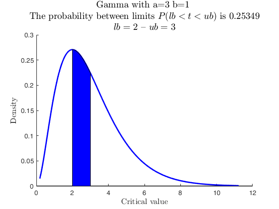
 Use with makedist, region inside.
Use with makedist, region inside.A Gamma with parameter values a = 3 and b = 1, in [2 3].
close all
pd = makedist('Gamma','a',3,'b',1);
specs  = [2 3];
region = 'inside';
[p, h] = distribspec(pd, specs, region);
pause(0.5);
Related Examples
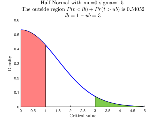
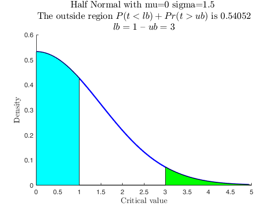
Use with makedist, using userColor for each outside region.
Use with makedist, using userColor for each outside region.
close all
rng('default')
pd = makedist('HalfNormal','mu',0,'sigma',1.5);
specs  = [1 3];
region = 'outside';
useColor = 'cg';
[p, h] = distribspec(pd, specs, region, 'userColor', useColor);
useColor = [1 0.5 0.5 ; 0.5 0.8 0.3];
[p, h] = distribspec(pd, specs, region, 'userColor', useColor);
cascade;
pause(0.5);
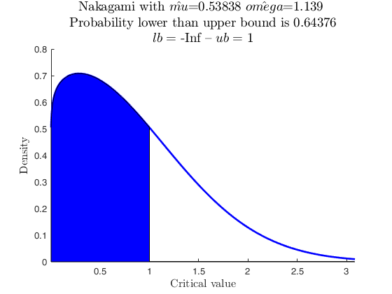
Use with distname.
Use with distname.
% A sample of n=100 elements extracted from a Nakagami.
close all
rng(12345);
distname    = 'Nakagami';
x           = random(distname,0.5,1,[100,1]);
pd          = struct;
pd.x        = x;
pd.distname = distname;
specs  = [-inf 1];
region = 'inside';
[p, h] = distribspec(pd, specs, region);
pause(0.5);
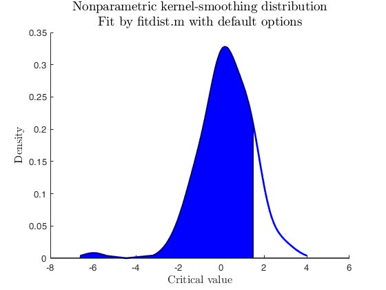
Use with a sample only.
Use with a sample only.
% A sample of n=100 elements extracted from a T(5) without distname.
close all
rng(12345);
x      = random('T',5,[100,1]);
specs  = [-inf 1.5];
region = 'inside';
[p, h] = distribspec(x, specs, region);
pause(0.5);
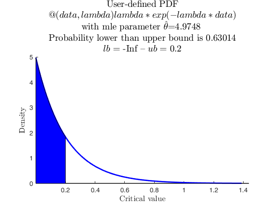
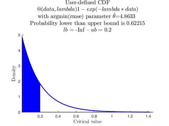
Sample from parametric used-defined distribution.
Sample from parametric used-defined distribution.
% Data from user-defined distribution, negative exponential with one parameter
close all
lambda = 5;
userpdf = @(data,lambda) lambda*exp(-lambda*data);
usercdf = @(data,lambda) 1-exp(-lambda*data);
rng(12345);
n = 500;
X = zeros(n,1);
u = rand(n,1);
for i = 1:numel(u)
fun  = @(x)integral(@(x)userpdf(x,lambda),eps,x) - u(i);
X(i) = fzero(fun,0.5);
% The previous two lines have the solution below, but exemplify the
% approach for a generic function without closed formula.
% X(i) = -(1/lambda)*log(1-u(i)); % p. 211 Mood Graybill and Boes
end
%Estimate the parameter lambda of the custom distribution.
parhat = mle(X,'pdf',userpdf,'cdf',usercdf,'start',0.05);
% plot data as a normalised histogram and the mle of the pdf
histogram(X,100,'Normalization','pdf');
hold on
plot(X,userpdf(X,parhat),'.')
title({['The sample generated by ' char(userpdf)] , ['with $\lambda=$' num2str(lambda)]} , 'Interpreter' , 'Latex');
hold off
% Set common specs and region settings
specs  = [-inf 0.2];
region = 'inside';
% Use distribspec with both usercdf and userpdf
pd          = struct;
pd.x        = X;
pd.distname = 'user';
pd.usercdf  = usercdf;
pd.userpdf  = userpdf;
[p, h] = distribspec(pd, specs, region);
% now with userpdf
pd          = struct;
pd.x        = X;
pd.distname = 'user';
pd.userpdf  = userpdf;
[p, h] = distribspec(pd, specs, region);
% and now with usercdf
pd          = struct;
pd.x        = X;
pd.distname = 'user';
pd.usercdf  = usercdf;
[p, h] = distribspec(pd, specs, region);
cascade;
pause(0.5);
User-defined function, with reduced number of evaluation points.
User-defined function, with reduced number of evaluation points.
% Data from user-defined distribution: Pareto (two parameters). This
% takes a while to complete, because of difficult integration (the
% function has singularities). Therefore, we reduce the ealuation
% points only to 50. In this case, being the function very smooth in
% the region of interest, the quality is not affected.
close all
alpha0  = 2;
xm0     = 4;
% data
rng(12345);
n = 500;
X = zeros(n,1);
u = rand(n,1);
for i = 1:numel(u)
X(i) = alpha0*(1-u(i)).^(-1/xm0);
end
% heaviside function
hvsd = @(y) [0.5*(y == 0) + (y > 0)];
userpdf0 = @(x) hvsd(x-xm0) .* (alpha0*4^alpha0) ./ (x.^(alpha0+1));
fplot(userpdf0);
xlim([-5 20]);
title({'Pareto distribution' , '$ hvsd(x-xm_{0}) \cdot (\alpha_{0} \cdot 4^{\alpha_{0}}) / (x^{\alpha_{0}+1})$' } , 'Interpreter','latex' , 'Fontsize' , 20);
pause(0.5);
userpdf = @(x, alpha) hvsd(x-4) .* ((alpha*4^alpha) ./ (x.^(alpha+1)));
%userpdf = @(x, alpha, xm) hvsd(x-xm) .* ((alpha*xm^alpha) ./ (x.^(alpha+1)));
%usercdf = @(x, alpha, xm) hvsd(x-xm) .* (1 - (xm./x).^alpha);
% Apply distribspec with userpdf
specs  = [5 10];
region = 'inside';
pd          = struct;
pd.x        = X;
pd.distname = 'user';
pd.userpdf  = userpdf;
pd.mleStart = mean(pd.x);
pd.mleLowerBound = pd.mleStart/2;
pd.mleUpperBound = pd.mleStart*2;
[p, h] = distribspec(pd, specs, region, 'evalPoints', 50);
cascade;
pause(0.5);
User-defined function starting from a default matlab distribution.
User-defined function starting from a default matlab distribution.
% Here the user takes one of the functions in makedist, possibly
% changing the number of parameters.
close all
alpha0  = 2;
xm0     = 4;
X = wblrnd(1,1,[1000,1]) + 10;
histogram(X,'Normalization','pdf');
title({'A sample from the weibull' , '$a=1, b=1, c=10$'},'Fontsize',20,'Interpreter','latex');
% A Weibull distribution with an extra parameter c
userpdf = @(x,a,b,c) wblpdf(x-c,a,b);
% Apply distribspec with userpdf
specs  = [11 12];
region = 'inside';
pd          = struct;
pd.x        = X;
pd.distname = 'user';
pd.userpdf  = userpdf;
pd.mleStart = [5 5 5];
pd.mleLowerBound = [0 0 -Inf];
pd.mleUpperBound = [Inf Inf min(X)];
% MLE parameters. The scale and shape parameters must be positive,
% and the location parameter must be smaller than the minimum of the
% sample data.
[p, h] = distribspec(pd, specs, region, 'evalPoints', 100);
cascade
pause(0.5);