distribspec
distribspec plots a probability density function between specification limits
Syntax
Description
distribspec generalises the MATLAB function normspec for plotting a selected probability density function by shading the portion inside or outside given limits.
Examples
Use with makedist, default settings.
A uniform distribution U(3,8), in [5,6].
a=3;
b=8;
pd=makedist('Uniform','Lower',a,'Upper',b);
distribspec(pd, [5 6], 'inside');
distribspec(pd, [5 6], 'outside');
cascade;
Use with makedist, default settings.
A standard normal distribution in [-1 1].
pd     = makedist('Normal');
specs  = [-1 1];
region = 'inside';
[p, h] = distribspec(pd, specs, region);
pause(0.5);
Related Examples
Use with makedist, region outside.
A Beta with parameter values a = 2 and b = 4, outside [0.2 0.4].
close all
pd = makedist('Beta','a',2,'b',4);
specs  = [0.2 0.4];
region = 'outside';
[p, h] = distribspec(pd, specs, region);
pause(0.5);
Use with makedist, specs with inf.
A Beta with parameter values a = 2 and b = 4, in [0.4 inf].
close all
pd = makedist('Beta','a',2,'b',4);
specs  = [0.4 inf];
region = 'inside';
[p, h] = distribspec(pd, specs, region);
pause(0.5);
Use with makedist, specs with -inf.
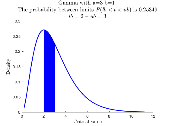
% A Gamma with parameter values a = 3 and b = 1, up to 2.
close all
pd = makedist('Gamma','a',3,'b',1);
specs  = [-inf 2];
region = 'inside';
[p, h] = distribspec(pd, specs, region);
% Without specification of region the default is inside, therefore,
% the output is identical
pd = makedist('Gamma','a',3,'b',1);
specs  = [-inf 2];
[p, h] = distribspec(pd, specs);
cascade;
pause(0.5);
Use with makedist, no specs.
A Gamma as above, without specification of specs: returns an error.
close all
pd = makedist('Gamma','a',3,'b',1);
region = 'inside';
try
[p, h] = distribspec(pd, [], region);
catch
disp(sprintf('%s\n\n%s\n%s',...
'Without specification of specs, distribspec returned this error:' , ...
'Error using distribspec' , ...
'Please provide valid lower and upper limits for the area to highlight'));
end
pause(0.5);
Use with makedist, specs outside support.
A Gamma with parameter values a = 3 and b = 1, up to -1. Nothing is colored.
close all
pd = makedist('Gamma','a',3,'b',1);
specs  = [-inf -1];
region = 'inside';
[p, h] = distribspec(pd, specs, region);
pause(0.5);
Use with makedist, using userColor.
% A Gamma as above, using userColor with standard one-character
% specification.
close all
pd = makedist('Gamma','a',3,'b',1);
specs  = [-inf 2];
region = 'inside';
[p, h] = distribspec(pd, specs, region, 'userColor','r');
% same, but using userColor with RGB triplet specification.
pd = makedist('Gamma','a',3,'b',1);
specs  = [-inf 2];
region = 'inside';
[p, h] = distribspec(pd, specs, region, 'userColor',[1 0.5 0.5]);
cascade;
pause(0.5);
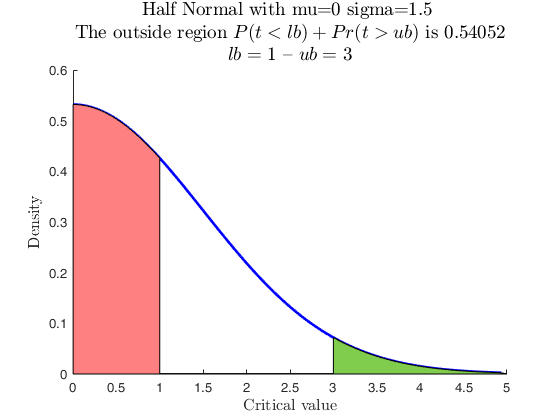
 Use with makedist, using userColor for each outside region.
 Use with makedist, using userColor for each outside region.
close all
rng('default')
pd = makedist('HalfNormal','mu',0,'sigma',1.5);
specs  = [1 3];
region = 'outside';
useColor = 'cg';
[p, h] = distribspec(pd, specs, region, 'userColor', useColor);
useColor = [1 0.5 0.5 ; 0.5 0.8 0.3];
[p, h] = distribspec(pd, specs, region, 'userColor', useColor);
cascade;
pause(0.5);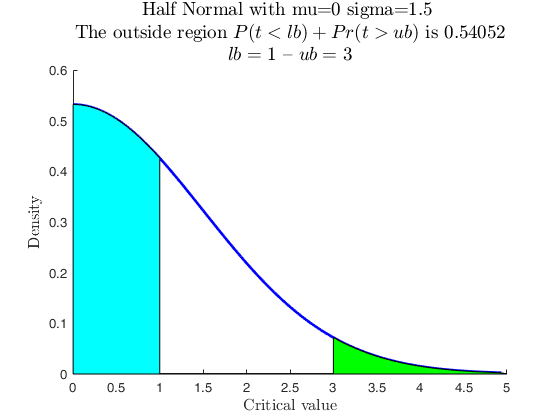
Use with makedist, using userColor with RGB triplet.
% A Half Normal using userColor with RGB triplet specification.
% The triplet is returned by FSColors.
close all
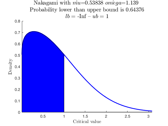
pd = makedist('HalfNormal','mu',0,'sigma',1.5);
specs  = [-inf 1];
region = 'inside';
RGB_vector = aux.FSColors.lightgrey.RGB;
[p, h] = distribspec(pd, specs, region, 'userColor',RGB_vector);
pause(0.5);
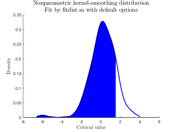
Sample from non-parametric used-defined distribution.
close all
% Data from user-defined distribution, Benford (non-parametric)
% no parameters to estimate
userpdf = @(n) log10(1 + 1./n);
usercdf = @(n) log10(1 + n);
% random sample from Benford
n = 5000;
u = rand(n,1);
X = 10.^u;
% Apply distribspec with userpdf
specs  = [-inf 5];
region = 'inside';
pd          = struct;
pd.x        = X;
pd.distname = 'user';
pd.userpdf  = userpdf;
[p, h] = distribspec(pd, specs, region);
pause(0.5);
 Sample from parametric used-defined distribution.
 Sample from parametric used-defined distribution.
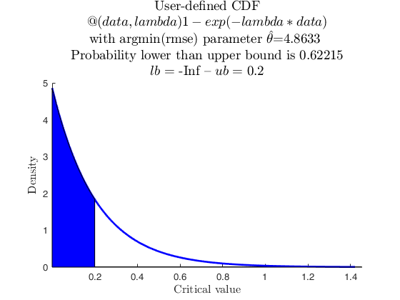
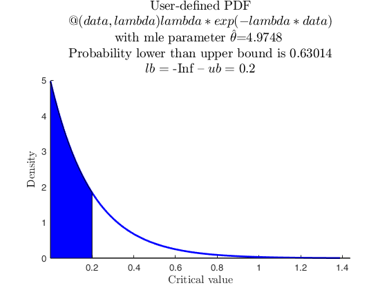
% Data from user-defined distribution, negative exponential with one parameter
close all
lambda = 5;
userpdf = @(data,lambda) lambda*exp(-lambda*data);
usercdf = @(data,lambda) 1-exp(-lambda*data);
rng(12345);
n = 500;
X = zeros(n,1);
u = rand(n,1);
for i = 1:numel(u)
fun  = @(x)integral(@(x)userpdf(x,lambda),eps,x) - u(i);
X(i) = fzero(fun,0.5);
% The previous two lines have the solution below, but exemplify the
% approach for a generic function without closed formula.
% X(i) = -(1/lambda)*log(1-u(i)); % p. 211 Mood Graybill and Boes
end
%Estimate the parameter lambda of the custom distribution.
parhat = mle(X,'pdf',userpdf,'cdf',usercdf,'start',0.05);
% plot data as a normalised histogram and the mle of the pdf
histogram(X,100,'Normalization','pdf');
hold on
plot(X,userpdf(X,parhat),'.')
title({['The sample generated by ' char(userpdf)] , ['with $\lambda=$' num2str(lambda)]} , 'Interpreter' , 'Latex');
hold off
% Set common specs and region settings
specs  = [-inf 0.2];
region = 'inside';
% Use distribspec with both usercdf and userpdf
pd          = struct;
pd.x        = X;
pd.distname = 'user';
pd.usercdf  = usercdf;
pd.userpdf  = userpdf;
[p, h] = distribspec(pd, specs, region);
% now with userpdf
pd          = struct;
pd.x        = X;
pd.distname = 'user';
pd.userpdf  = userpdf;
[p, h] = distribspec(pd, specs, region);
% and now with usercdf
pd          = struct;
pd.x        = X;
pd.distname = 'user';
pd.usercdf  = usercdf;
[p, h] = distribspec(pd, specs, region);
cascade;
pause(0.5);
 User-defined function, with reduced number of evaluation points.
 User-defined function, with reduced number of evaluation points.
% Data from user-defined distribution: Pareto (two parameters). This
% takes a while to complete, because of difficult integration (the
% function has singularities). Therefore, we reduce the ealuation
% points only to 50. In this case, being the function very smooth in
% the region of interest, the quality is not affected.
close all
alpha0  = 2;
xm0     = 4;
% data
rng(12345);
n = 500;
X = zeros(n,1);
u = rand(n,1);
for i = 1:numel(u)
X(i) = alpha0*(1-u(i)).^(-1/xm0);
end
% heaviside function
hvsd = @(y) [0.5*(y == 0) + (y > 0)];
userpdf0 = @(x) hvsd(x-xm0) .* (alpha0*4^alpha0) ./ (x.^(alpha0+1));
fplot(userpdf0);
xlim([-5 20]);
title({'Pareto distribution' , '$ hvsd(x-xm_{0}) \cdot (\alpha_{0} \cdot 4^{\alpha_{0}}) / (x^{\alpha_{0}+1})$' } , 'Interpreter','latex' , 'Fontsize' , 20);
pause(0.5);
userpdf = @(x, alpha) hvsd(x-4) .* ((alpha*4^alpha) ./ (x.^(alpha+1)));
%userpdf = @(x, alpha, xm) hvsd(x-xm) .* ((alpha*xm^alpha) ./ (x.^(alpha+1)));
%usercdf = @(x, alpha, xm) hvsd(x-xm) .* (1 - (xm./x).^alpha);
% Apply distribspec with userpdf
specs  = [5 10];
region = 'inside';
pd          = struct;
pd.x        = X;
pd.distname = 'user';
pd.userpdf  = userpdf;
pd.mleStart = mean(pd.x);
pd.mleLowerBound = pd.mleStart/2;
pd.mleUpperBound = pd.mleStart*2;
[p, h] = distribspec(pd, specs, region, 'evalPoints', 50);
cascade;
pause(0.5);
 User-defined function starting from a default matlab distribution.
 User-defined function starting from a default matlab distribution.
% Here the user takes one of the functions in makedist, possibly
% changing the number of parameters.
close all
alpha0  = 2;
xm0     = 4;
X = wblrnd(1,1,[1000,1]) + 10;
histogram(X,'Normalization','pdf');
title({'A sample from the weibull' , '$a=1, b=1, c=10$'},'Fontsize',20,'Interpreter','latex');
% A Weibull distribution with an extra parameter c
userpdf = @(x,a,b,c) wblpdf(x-c,a,b);
% Apply distribspec with userpdf
specs  = [11 12];
region = 'inside';
pd          = struct;
pd.x        = X;
pd.distname = 'user';
pd.userpdf  = userpdf;
pd.mleStart = [5 5 5];
pd.mleLowerBound = [0 0 -Inf];
pd.mleUpperBound = [Inf Inf min(X)];
% MLE parameters. The scale and shape parameters must be positive,
% and the location parameter must be smaller than the minimum of the
% sample data.
[p, h] = distribspec(pd, specs, region, 'evalPoints', 100);
cascade
pause(0.5);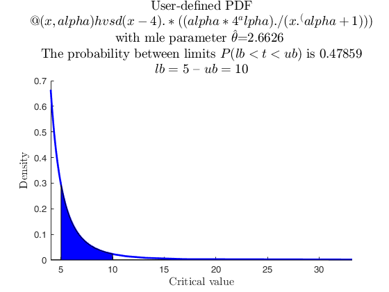
Example with the Chi2 distribution with v degrees of freedom.
Set the degrees of freedom.
v=6;
% Create the Chi2 with v degrees of freedom
pd = makedist('Gamma','a',v/2,'b',2);
p= distribspec(pd,[icdf(pd,0.05)  icdf(pd,0.95)])
Input Arguments
pd — can be one of the following.
- A probability density object returned by makedist.
- A structure containing two fields: (i) pd.distname, a character array with a valid distribution name (all those accepted by makedist);
(ii) pd.x, a numeric vector containing the data sample to be used to estimate the parameters of the distribution.
- A structure containing three fields with these features: (i) pd.distname containing the character array 'user'.
(ii) pd.userpdf containing a user defined function handle expressing the probability density function;
(iii) pd.usercdf containing a user defined function handle expressing the cumulative density function;
(iv) pd.x, a numeric vector containing the data sample to be used to estimate the parameters of the user-defined distribution. The estimation is done by maximum likelihood using MATLAB function mle.
- A numeric vector containing a sample used to fit a probability distribution object with nonparametric kernel-smoothing.
Other optional fields can be set to help improving the speed and quality of the results obtained for user-defined distributions.
In particular, when a data sample is provided in pd.x, the user can add to structue pd additional fields to control the estimation of the distribution parameters made by distribspec using matlab function mle: - pd.mleStart, used as initial parameter values. The choice of the starting point is often crucial for the convergence of mle. If the initial parameter values are far from the true maximum likelihood estimate, we can obtain underflow in the distribution functions and infinite loglikelihoods.
A reasonable choice for the initial value of a location parameter could be pd.mleStart = mean(pd.x). Similarily, for a scale parameter we could set pd.mleStart = std(pd.x).
- pd.mleLowerBound, which indicates Lower bounds for distribution parameters. For example, if we trust pd.mleStart, we could set pd.mleLowerBound = pd.mleStart/2.
- pd.mleUpperBound, which indicates teh Upper bounds for distribution parameters. Along the previous case, we could set pd.mleUpperBound = pd.mleStart*2;
Data Types: single| double
specs — the lower and upper limits of the shading area.
Two element
vector.
If there is no lower limit, then specs(1)=-Inf. If there is no upper limit, then specs(2)=Inf.
Data Types: single| double
region — the region to shade.
Character array.
It can be either the portion 'inside' or 'outside' of the spec limits.
Data Types: single| double
Name-Value Pair Arguments
Specify optional comma-separated pairs of Name,Value arguments.
Name is the argument name and Value
is the corresponding value. Name must appear
inside single quotes (' ').
You can specify several name and value pair arguments in any order as
Name1,Value1,...,NameN,ValueN.
 'userColor', 'b'
, 'evalPoints', [1.5 3.2]
userColor
—The color of the shaded area.character, 2-element character array, RGB triplet, 2-row RGB triplet.
The character can be any of the LineSpec colors properties of MATLAB plot function. The RGB triplet specification is defined as usual, that is with three numbers taking values in [0 1]: to generate the triplet, the user can use FSDA function FSColors. For example you can use 'userColor', 'r', or 'userColor', 'rb' or 'userColor', FSColors.lightgrey.RGB, or 'userColor', [FSColors.lightgrey.RGB ; FSColors.grey.RGB]
Example: 'userColor', 'b'
Data Types: character, character array, 3-element
array for a RGB triplet,2-row with RGB triplets
evalPoints
—Evaluation points.scalar.
Number of points where the the pdf is evaluated and plotted. Default is 1000. The default is ok for most cases. However, when distribspec appears too slow, try reducing the number of evaluation points. If on the contrary the plot looks not sufficiently smooth, increase the number of evaluation points.
Example: 'evalPoints', [1.5 3.2]
Data Types: scalar or array
