mcd
mcd computes Minimum Covariance Determinant
Syntax
Description
Examples
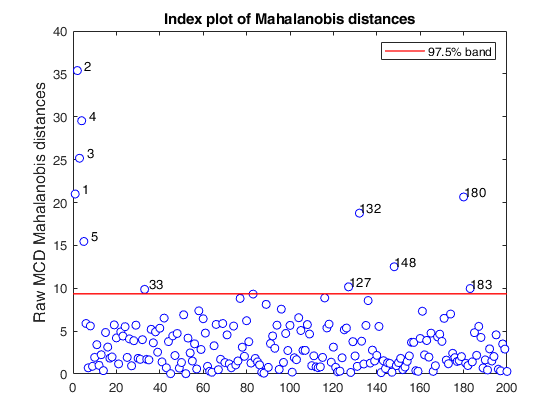
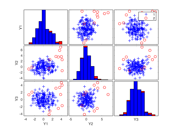
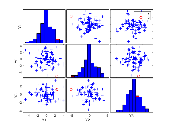
 mcd with optional arguments.
mcd with optional arguments.
n=200;
v=3;
randn('state', 123456);
Y=randn(n,v);
% Contaminated data
Ycont=Y;
Ycont(1:5,:)=Ycont(1:5,:)+3;
RAW=mcd(Ycont,'plots',1);
Total estimated time to complete MCD: 0.34 seconds

Related Examples
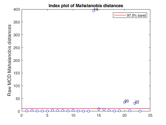
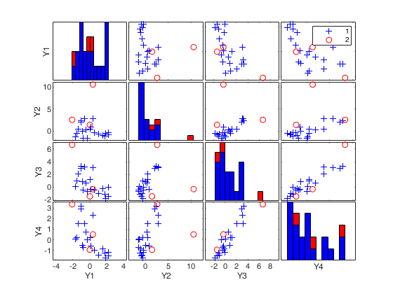
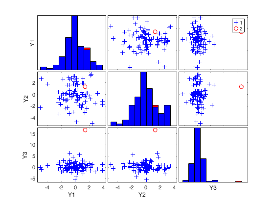
mcd applied to the aircraft data (default plots).
mcd applied to the aircraft data (default plots).See Pison et al. 2002, Metrika.
X = load('aircraft.txt');
Y = X(:,1:end-1);
[RAW,RES] = mcd(Y,'bdp',0.25,'plots',1);
Total estimated time to complete MCD: 0.14 seconds
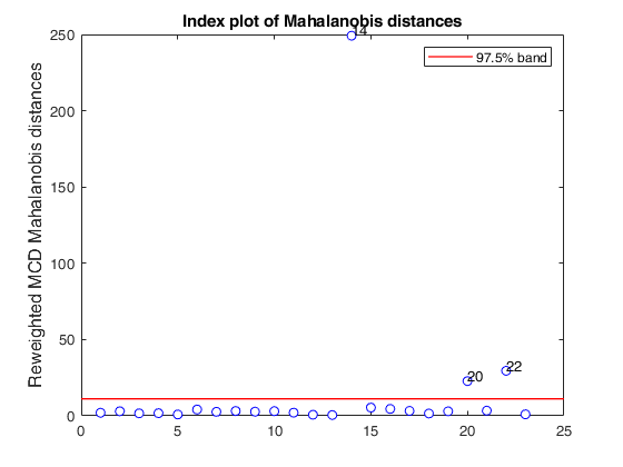

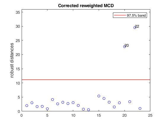
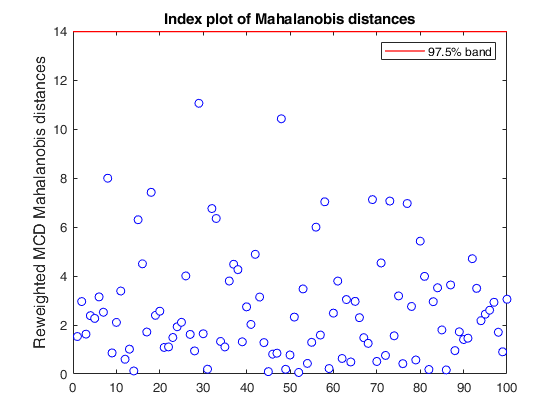
mcd applied to the aircraft data (plots using the scale of Pison et al).
mcd applied to the aircraft data (plots using the scale of Pison et al).See Pison et al. 2002, Metrika.
X = load('aircraft.txt');
Y = X(:,1:end-1);
[RAW,REW] = mcd(Y,'bdp',0.25,'ysaveRAW',1);
v=size(Y,2);
% Compare the following figure with panel (b) of Fig. 8 of Pison et al.
ylimy=[0 36];
malindexplot(RAW.md,v,'conflev',0.975,'laby','robust distances','numlab',RAW.outliers,'ylimy',ylimy);
title('Corrected MCD')
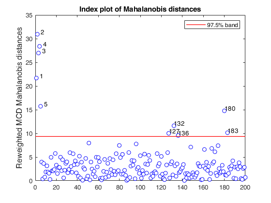
% Compare the following figure with panel (4) of Fig. 8 of Pison et al.
ylimy=[0 36];
malindexplot(REW.md,v,'conflev',0.975,'laby','robust distances','numlab',REW.outliers,'ylimy',ylimy);
title('Corrected reweighted MCD')
Total estimated time to complete MCD: 0.04 seconds
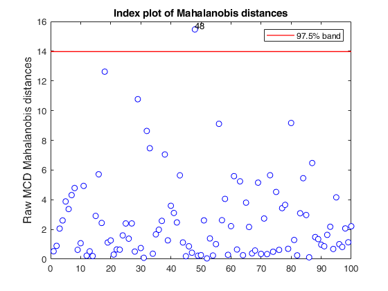
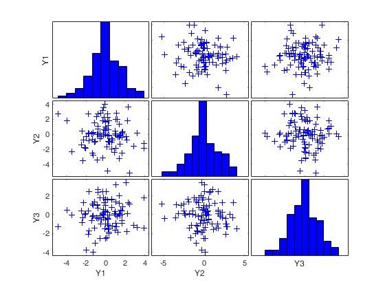
mcd with data from the Student-t model.
mcd with data from the Student-t model.
randn('state', 123456);
n  = 100;
v  = 3;
nu = 5;
% sample from the T
Yt = random('T',nu,[n,v]);
Yn = random('Normal',0,1,[n,v]);
Y = Yt;
% mcd with the T-model
RAWt = mcd(Y,'modelT',nu,'plots',1);
% mcd with the Normal-model
% RAWn = mcd(Y,'plots',1);
Total estimated time to complete MCD: 0.06 seconds
Input Arguments
Output Arguments
More About
References
Maronna, R.A., Martin D. and Yohai V.J. (2006), "Robust Statistics, Theory and Methods", Wiley, New York.
Acknowledgements
This function follows the lines of MATLAB/R code developed during the years by many authors. In particular, parts of the code rely on the LIBRA mcd implementation of Hubert and Verboven. For more details, see: https://wis.kuleuven.be/stat/robust/papers/2005/LIBRA.pdf and the R library Robustbase http://robustbase.r-forge.r-project.org/ The core of our routines, e.g. the resampling approach, however, has been completely redesigned, with considerable increase of the computational performance. Note that, for the moment, FSDA does not adopt the 'divide and conquer' partitioning method proposed by Rousseeuw and Van Driessen to speed up computations for large datasets. This partitioning method is applied in the R and LIBRA implementations of the mcd.