mmdrsplot
mmdrsplot plots the trajectories of minimum Mahalanobis distances from different starting points
Syntax
Description
Example of mmdrsplot with all the default options.brushedUnits
=mmdrsplot(out)
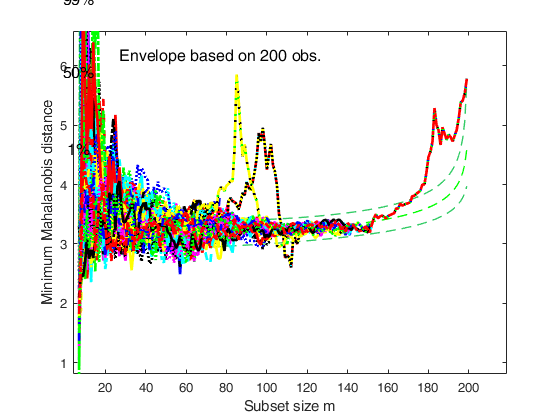
Example of the use of function mmdrsplot with personalized envelopes.brushedUnits
=mmdrsplot(out,
Name, Value)
[
Interactive_example
mmdrsplot with option dataooltip.brushedUnits,
BrushedUnits]
=mmdrsplot(___)
Examples
 Example of mmdrsplot with all the default options.
Example of mmdrsplot with all the default options.
load('swiss_banknotes');
Y=swiss_banknotes{:,:};
[fre]=unibiv(Y);
%create an initial subset with the 4 observations, which fell the smallest
%number of times outside the robust bivariate ellipses, and with the
%lowest Mahalanobis Distance.
fre=sortrows(fre,[3 4]);
m0=20;
bs=fre(1:m0,1);
[outeda]=FSMeda(Y,bs);
[out]=FSMmmdrs(Y,'bsbsteps',0,'cleanpool',0,'nsimul',80);
mmdrsplot(out);
Example of the use of function mmdrsplot with personalized envelopes.
load('swiss_banknotes');
Y=swiss_banknotes{:,:};
[fre]=unibiv(Y);
fre=sortrows(fre,[3 4]);
m0=20;
bs=fre(1:m0,1);
[outeda]=FSMeda(Y,bs);
[out]=FSMmmdrs(Y,'bsbsteps',0,'cleanpool',0,'nsimul',80);
mmdrsplot(out,'quant',[0.99;0.9999]);
Interactive example 1.
mmdrsplot with option dataooltip.
%Example of the use of function mmdrsplot with datatooltip passed as
%scalar (that is using default options for datacursor (i.e.
%DisplayStyle =window)
load('swiss_banknotes');
Y=swiss_banknotes{:,:};
[fre]=unibiv(Y);
fre=sortrows(fre,[3 4]);
m0=20;
bs=fre(1:m0,1);
[outeda]=FSMeda(Y,bs);
[out]=FSMmmdrs(Y,'bsbsteps',0,'cleanpool',0,'nsimul',80);
mmdrsplot(out,'datatooltip',1);
Related Examples
Interactive example 2.
mmdrsplot with option dataooltip passed as structure.
%Example of the use of function mmdrsplot with datatooltip passed as
%structure
load('swiss_banknotes');
Y=swiss_banknotes{:,:};
[fre]=unibiv(Y);
fre=sortrows(fre,[3 4]);
m0=20;
bs=fre(1:m0,1);
[outeda]=FSMeda(Y,bs);
[out]=FSMmmdrs(Y,'bsbsteps',0,'cleanpool',0,'nsimul',80);
clear tooltip
tooltip.SnapToDataVertex='on'
tooltip.DisplayStyle='datatip'
mmdrsplot(out,'datatooltip',tooltip);
Interactive example 3.
Example of the use of option databrush.
load('swiss_banknotes');
Y=swiss_banknotes{:,:};
[fre]=unibiv(Y);
fre=sortrows(fre,[3 4]);
m0=20;
bs=fre(1:m0,1);
[outeda]=FSMeda(Y,bs);
[out]=FSMmmdrs(Y,'bsbsteps',0,'cleanpool',0,'nsimul',80);
mmdrsplot(out,'databrush',1);
Interactive example 4.
Two groups with approximately the same number of units.
close all
rng('default')
rng(10);
n1=100;
n2=100;
v=3;
Y1=rand(n1,v);
Y2=rand(n2,v)+1;
Y=[Y1;Y2];
group=[ones(n1,1);2*ones(n2,1)];
spmplot(Y,group);
title('Two simulated groups')
Y=[Y1;Y2];
close all
% parfor of Parallel Computing Toolbox is used (if present in current computer)
% and pool is not cleaned after the execution of the random starts
% The number of workers which is used is the one specified
% in the local/current profile
[out]=FSMmmdrs(Y,'nsimul',100,'init',10,'plots',1,'cleanpool',0);
ylim([2 5])
disp('The two peaks in the trajectories of minimum Mahalanobis distance (mmd).')
disp('clearly show the presence of two groups.')
disp('The decrease after the peak in the trajectories of mmd is due to the masking effect.')
mmdrsplot(out,'databrush',1)
Interactive example 5.
Example of the use of option databrush.
% Selected units are also highlighted in the malfwdplot.
load('swiss_banknotes');
Y=swiss_banknotes{:,:};
out=FSMmmdrs(Y,'bsbsteps',0,'cleanpool',0,'nsimul',80);
outEDA=FSMeda(Y,1:10,'init',20,'scaled',1);
malfwdplot(outEDA)
databrush=struct;
% If persist is 'off' after each selection, all trajectories except
% those selected in the current iteration are plotted in
% greysh color. If persist is 'on' after each selection, trajectories
% never selected in any iteration are plotted in greysh color.
databrush.persist='on';
% outV is the vector of all selected units during brushing
% outM is a matrix, each column contains the groups of selected units
% at each brushing action
[outV, outM]=mmdrsplot(out,'databrush',databrush)
Input Arguments
out — Structure containing the following fields.
out.mmdrs = a matrix of size (n-ninit)-by-(nsimul+1)containing the
monitoring of minimum Mahalanobis distance
in each step of the forward search for each of the nsimul random starts.
The first column of mmdrs must contain the fwd search index.
This matrix can be created using function FSMmmdrs.
out.BBrs = 3D array of size n-by-n-(init)-by-nsimul containing units forming subset for each random start.
This field is necessary if datatooltip is true or databrush is not empty.
out.Y = n-by-v matrix containing the original datamatrix This field is necessary if datatooltip is true or databrush is not empty.
Data Types: single| double
Name-Value Pair Arguments
Specify optional comma-separated pairs of Name,Value arguments.
Name is the argument name and Value
is the corresponding value. Name must appear
inside single quotes (' ').
You can specify several name and value pair arguments in any order as
Name1,Value1,...,NameN,ValueN.
 'quant',[0.01 0.99]
, 'envm',n
, 'xlimx',[20 100]
, 'ylimy',[2 6]
, 'lwdenv',2
, 'tag','mymmdrs'
, 'datatooltip',1
, 'databrush',1
, 'FontSize',14
, 'SizeAxesNum',14
, 'nameY',{'Age','Income','Married','Profession'}
, 'lwd',3
, 'namey','Plot title'
, 'labx','Subset size m'
, 'laby','mmd'
, 'labenv',false
, 'scaled',0
quant
—quantiles for which envelopes have
to be computed.vector.
1 x k vector containing quantiles for which envelopes have to be computed. The default is to produce 1%, 50% and 99% envelopes.
Example: 'quant',[0.01 0.99]
Data Types: double
envm
—sample size to use.scalar.
Scalar which specifies the size of the sample which is used to superimpose the envelope. The default is to add an envelope based on all the observations (size n envelope).
Example: 'envm',n
Data Types: double
xlimx
—min and max for x axis.vector.
vector with two elements controlling minimum and maximum on the x axis.
Default value is mmd(1,1)-3 and mmd(end,1)*1.3
Example: 'xlimx',[20 100]
Data Types: double
ylimy
—min and max for x axis.vector.
Vector with two elements controlling minimum and maximum on the y axis.
Default value is min(mmd(:,2)) and max(mmd(:,2));
Example: 'ylimy',[2 6]
Data Types: double
lwdenv
—Line width.scalar.
Scalar which controls the width of the lines associated with the envelopes.
Default is lwdenv=1
Example: 'lwdenv',2
Data Types: double
tag
—plot handle.string.
String which identifies the handle of the plot which is about to be created. The default is to use tag 'pl_mmdrs'. Notice that if the program finds a plot which has a tag equal to the one specified by the user, then the output of the new plot overwrites the existing one in the same window else a new window is created.
Example: 'tag','mymmdrs'
Data Types: char
datatooltip
—interactive clicking.empty value (default) | structure.
If datatooltip is not empty the user can use the mouse in order to have information about the unit selected, the step in which the unit enters the search and the associated label. If datatooltip is a structure, it is possible to control the aspect of the data cursor (see function datacursormode for more details or the examples below). The default options of the structure are DisplayStyle='Window' and SnapToDataVertex='on'.
Example: 'datatooltip',1
Data Types: empty value, numeric or structure
databrush
—interactive mouse brushing.empty value (default), scalar | structure.
DATABRUSH IS AN EMPTY VALUE .
If databrush is an empty value (default), no brushing is done. The activation of this option (databrush is a scalar or a structure) enables the user to select a set of trajectories in the current plot and to see them highlighted in the spm (notice that if the spm does not exist it is automatically created).
In addition, units forming subset in the selected steps selected trajectories can be highlighted in the monitoring MD plot Note that the window style of the other figures is set equal to that which contains the monitoring residual plot. In other words, if the monitoring residual plot is docked all the other figures will be docked too.
DATABRUSH IS A SCALAR.
If databrush is a scalar the default selection tool is a rectangular brush and it is possible to brush only once (that is persist='').
DATABRUSH IS A STRUCTURE.
If databrush is a structure, it is possible to use all optional arguments of function selectdataFS and the following optional argument: persist. Persist is an empty value or a scalar containing the strings 'on' or 'off' If persist = 'on' or 'off' brusing can be done as many time as the user requires. If persist='on' then the unit(s) currently brushed are added to those previously brushed. If persist='off' every time a new brush is performed units previously brushed are removed. The default value of persist is '' that is brushing is allowed only once. If persist is 'on' it is possible, every time a new brushing is done, to use a different color for the brushed units labeladd. If this option is '1', we label the units of the last selected group with the unit row index in matrices X and y. The default value is labeladd='', i.e. no label is added.
Remark: if databrush is a struct, it is possible to specify all optional arguments of function selectdataFS inside the curly brackets of option databrush.
Example: 'databrush',1
Data Types: single | double | struct
FontSize
—Size of axes labels.scalar.
Scalar which controls the fontsize of the labels of the axes.
Default value is 12.
Example: 'FontSize',14
Data Types: single | double
SizeAxesNum
—Size of axes numbers.scalar.
Scalar which controls the fontsize of the numbers of the axes.
Default value is 10.
Example: 'SizeAxesNum',14
Data Types: single | double
nameY
—Regressors names.cell array of strings.
Cell array of strings of length v containing the labels of the varibales of the original data matrix. If it is empty (default) the sequence Y1, ..., Yp will be created automatically.
Example: 'nameY',{'Age','Income','Married','Profession'}
Data Types: cell
lwd
—Curves line width.scalar.
Scalar which controls linewidth of the curve which contains the monitoring of minimum Mahalanobis distance.
Default line width=2
Example: 'lwd',3
Data Types: single | double
titl
—main title.character.
A label for the title (default: '').
Example: 'namey','Plot title'
Data Types: char
labx
—x axis title.character.
A label for the x-axis (default: 'Subset size m').
Example: 'labx','Subset size m'
Data Types: char
laby
—y axis title.character.
A label for the y-axis (default: 'Minimum Mahalnobis distance').
Example: 'laby','mmd'
Data Types: char
labenv
—label the envelopes.boolean.
If labenv is true (default) labels of the confidence envelopes which are used are added on the y axis.
Example: 'labenv',false
Data Types: boolean
scaled
—scaled or unscaled envelopes.boolean.
Use reference envelopes scaled or unscaled).
If scaled=1 the envelopes are produced for scaled Mahalanobis distances (no consistency factor is applied) else the traditional consistency factor is applied Default is to use unscaled envelopes.
Example: 'scaled',0
Data Types: char
Output Arguments
brushedUnits —List of the
units which are inside subset in the trajectories which
have been brushed using option databrush.
brushed units. Vector. Vector
If option databrush has not been used, brushedUnits will be an empty value.
BrushedUnits —brushed units.
Matrix
Matrix of size r-by-numBrushingActions which contains in column j the brushed units after jth brushing.
If during jth brushing action the number of brushed units is the last r-s units of column j are set to 0.
References
Atkinson, A.C., Riani, M. and Cerioli, A. (2004), "Exploring multivariate data with the forward search", Springer Verlag, New York.