FSMmmdrs

FSMmmdrs performs random start monitoring of minimum Mahalanobis distance

Syntax

Description

The trajectories originate from many different random initial subsets and provide information on the presence of groups in the data. Groups are investigated by monitoring the minimum Mahalanobis distance outside the FS subset.

example

out =FSMmmdrs(Y) Two groups with approximately same units.

example

out =FSMmmdrs(Y, Name, Value) Two groups with approximately same units (larger sizes).

Examples

expand all

  • Two groups with approximately same units.
  • We start with an example with simulated data with two groups with roughly the same number of observations

    close all
    rng('default')
    rng(10);
    n1=100;
    n2=100;
    v=3;
    Y1=rand(n1,v);
    Y2=rand(n2,v)+1;
    Y=[Y1;Y2];
    group=[ones(n1,1);2*ones(n2,1)];
    spmplot(Y,group);
    title('Two simulated groups')
    Y=[Y1;Y2];
    close all
    % parfor of Parallel Computing Toolbox is used (if present in current computer)
    % and pool is cleaned after the execution of the random starts
    % The number of workers which is used is the one specified
    % in the local/current profile
    [out]=FSMmmdrs(Y,'nsimul',100,'init',10,'plots',1);
    ylim([2 5])
    disp('The two peaks in the trajectories of minimum Mahalanobis distance (mmd).')
    disp('clearly show the presence of two groups.')
    disp('The decrease after the peak in the trajectories of mmd is due to the masking effect.')
    Click here for the graphical output of this example (link to Ro.S.A. website).

  • Two groups with approximately same units (larger sizes).
  • Same example as before but now the values of n1 and n2 (size of the two groups) have been increased.

    close all
    rng('default')
    rng(10);
    n1=200;
    n2=170;
    v=3;
    Y1=rand(n1,v);
    Y2=rand(n2,v)+1;
    Y=[Y1;Y2];
    group=[ones(n1,1);2*ones(n2,1)];
    spmplot(Y,group);
    title('Two simulated groups')
    Y=[Y1;Y2];
    close all
    % parfor of Parallel Computing Toolbox is used (if present in current
    % computer) and pool is not cleaned after
    % the execution of the random starts
    [out]=FSMmmdrs(Y,'nsimul',100,'init',10,'plots',1);
    disp('The two peaks in the trajectories of minimum Mahalanobis distance (mmd).')
    disp('clearly show the presence of two groups.')
    disp('The decrease after the peak in the trajectories of mmd is due to the masking effect.')

    Related Examples

    expand all

  • Two groups (different sizes).
  • Same example as before but now there is one group which has a size much greater than the other (n1=60 and n2=150). In this case it is possible to see that there is a trajectory of minimum Mahalanobis residual which goes outside the envelope in steps 60-80. This corresponds to the searches initialized using the units coming from the smaller group. Note that due to the partial overlapping after the peak in steps 80-100 there is a gradual decrease. When m is around 140, most of the units from this group tend to get out of the subset.

    % Therefore the value of mmd becomes much smaller than it should be.
    % Please note the dip around step m=140, which is due to entrance of the
    % units of the second larger group. This trajectory just after the dip
    % collapses into the trajectory which starts from the second group.
    % Please use
    % mdrrsplot with option databrush in order to explore the units
    % belonging to subset. Here we limit ourselves to notice that around m
    % =180 all the units from second group are included into subset (plus
    % some of group 1 given that the two groups partially overlap). Also
    % notice once again the decrease in the unique trajectory of minimum
    % Mahalanobis residual after m around 180 which is due to the entry of the
    % units of the first smaller group.
    close all
    rng('default')
    rng(10);
    n1=60;
    n2=150;
    v=3;
    Y1=randn(n1,v);
    Y2=randn(n2,v)+3;
    Y=[Y1;Y2];
    group=[ones(n1,1);2*ones(n2,1)];
    spmplot(Y,group);
    title('Two simulated groups')
    Y=[Y1;Y2];
    figure
    % parfor of Parallel Computing Toolbox is used (if present in current
    % computer). Parallel pool is not closed after the execution of the random starts
    [out]=FSMmmdrs(Y,'nsimul',100,'init',10,'plots',1);

  • Fishery example.
  • Random start for fishery dataset: just store information about the units forming subset for each random start at specified steps

    load('fishery.txt');
    Y=fishery(:,1:2);
    figure
    [out]=FSMmmdrs(Y,'nsimul',100,'init',10,'plots',1,'bsbsteps',[10 300 600]);
    % sum(~isnan(out.BBrs(:,1,1)))
    %
    % ans =
    %
    %     10
    %
    % sum(~isnan(out.BBrs(:,2,1)))
    %
    % ans =
    %
    %    300
    %
    % sum(~isnan(out.BBrs(:,3,1)))
    %
    % ans =
    %
    %    600

    Input Arguments

    expand all

    Y — Input data. Matrix.

    n x v data matrix; n observations and v variables. Rows of Y represent observations, and columns represent variables.

    Missing values (NaN's) and infinite values (Inf's) are allowed, since observations (rows) with missing or infinite values will automatically be excluded from the computations.

    Data Types: single|double

    Name-Value Pair Arguments

    Specify optional comma-separated pairs of Name,Value arguments. Name is the argument name and Value is the corresponding value. Name must appear inside single quotes (' '). You can specify several name and value pair arguments in any order as Name1,Value1,...,NameN,ValueN.

    Example: 'init',10 , 'bsbsteps',[10 20 30] , 'nsimul',1000 , 'nocheck',1 , 'plots',0 , 'numpool',8 , 'cleanpool',1 , 'msg',0

    init —scalar, specifies the point where to initialize the search and start monitoring the required diagnostics.if not specified, it is set equal to p+1.

    Example: 'init',10

    Data Types: double

    bsbsteps —vector which specifies for which steps of the fwd search it is necessary to save the units forming subset for each random start.if bsbsteps is 0 for each random start we store the units forming subset in all steps.

    The default is store the units forming subset in all steps if n<=500 else to store the units forming subset at step init and steps which are multiple of 100. For example, if n=753 and init=6, units forming subset are stored for m=init, 100, 200, 300, 400, 500 and 600.

    REMARK: vector bsbsteps must contain numbers from init to n. if min(bsbsteps)<init a warning message will appear on the screen.

    Example: 'bsbsteps',[10 20 30]

    Data Types: double

    nsimul —scalar, number of random starts.default value=200.

    Example: 'nsimul',1000

    Data Types: double

    nocheck —It controls whether to perform checks on matrix Y.scalar.

    If nocheck is equal to 1 no check is performed.

    As default nocheck=0.

    Example: 'nocheck',1

    Data Types: double

    plots —scalar.if equal to one a plot of random starts minimum Mahalanobis residual appears on the screen with 1%, 50% and 99% confidence bands else (default) no plot is shown.

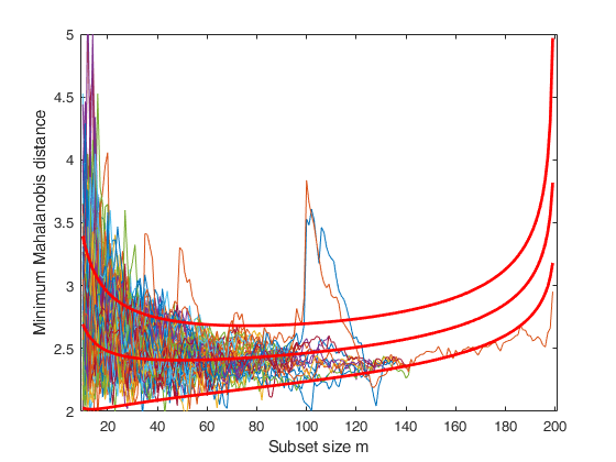
    The scale (ylim) for the y axis is defined as follows: ylim(2) is the maximum between the values of mmd in steps [n*0.2 n] and the final value of the 99 per cent envelope multiplied by 1.1.

    ylim(1) is the minimum between the values of mmd in steps [n*0.2 n] and the 1 per cent envelope multiplied by 0.9.

    Remark: the plot which is produced is very simple. In order to control a series of options in this plot (including the y scale) and in order to connect it dynamically to the other forward plots it is necessary to use function mmdrsplot.

    Example: 'plots',0

    Data Types: double

    numpool —scalar.if numpool > 1, the routine automatically checks if the Parallel Computing Toolbox is installed and distributes the random starts over numpool parallel processes.

    If numpool <= 1, the random starts are run sequentially. By default, numpool is set equal to the number of physical cores available in the CPU (this choice may be inconvenient if other applications are running concurrently). The same happens if the numpool value chosen by the user exceeds the available number of cores.

    REMARK : up to R2013b, there was a limitation on the maximum number of cores that could be addressed by the parallel processing toolbox (8 and, more recently, 12).

    From R2014a, it is possible to run a local cluster of more than 12 workers.

    REMARK : Unless you adjust the cluster profile, the default maximum number of workers is the same as the number of computational (physical) cores on the machine.

    REMARK : In modern computers the number of logical cores is larger than the number of physical cores. By default, MATLAB is not using all logical cores because, normally, hyper-threading is enabled and some cores are reserved to this feature.

    REMARK : It is because of Remarks 3 that we have chosen as default value for numpool the number of physical cores rather than the number of logical ones. The user can increase the number of parallel pool workers allocated to the multiple start monitoring by: - setting the NumWorkers option in the local cluster profile settings to the number of logical cores (Remark 2). To do so go on the menu "Home|Parallel|Manage Cluster Profile" and set the desired "Number of workers to start on your local machine".

    - setting numpool to the desired number of workers;

    Therefore, *if a parallel pool is not already open*, UserOption numpool (if set) overwrites the number of workers set in the local/current profile. Similarly, the number of workers in the local/current profile overwrites default value of 'numpool' obtained as feature('numCores') (i.e. the number of physical cores).

    Example: 'numpool',8

    Data Types: double

    cleanpool —Boolean.cleanpool is 1 (true) if the parallel pool has to be cleaned after the execution of the random starts.

    Otherwise it is 0 (false). The default value of cleanpool is false. Clearly this option has an effect just if previous option numpool is > 1.

    Example: 'cleanpool',1

    Data Types: boolean

    msg —Level of output to display.scalar.

    Scalar which controls whether to display or not messages about random start progress. More precisely, if previous option numpool>1, then a progress bar is displayed, on the other hand a message will be displayed on the screen when 10%, 25%, 50%, 75% and 90% of the random starts have been accomplished.

    REMARK: in order to create the progress bar when nparpool>1 the program writes on a temporary .txt file in the folder where the user is working. Therefore it is necessary to work in a folder where the user has write permission. If this is not the case and the user (say) is working without write permission in folder C:\Program Files\MATLAB the following message will appear on the screen: Error using ProgressBar (line 57) Do you have write permissions for C:\Program Files\MATLAB?

    Example: 'msg',0

    Data Types: double

    Output Arguments

    expand all

    out — description Structure

    A structure containing the following fields:

    Value Description
    mmdrs

    Minimum Mahalanobis distance. Matrix.

    (n-init)-by-(nsimul+1) matrix which contains the monitoring of minimum Mahalanobis distance at each step of the forward search for each random start.

    1st col = fwd search index (from init to n-1);

    2nd col = minimum Mahalanobis distance for random start 1;

    ...;

    nsimul+1 col = minimum deletion residual for random start nsimul.

    BBrs

    units belonging to the subset. 3D array.

    Units belonging to the subset at the steps specified by input option bsbsteps.

    If bsbsteps=0 BBrs has size n-by-(n-init+1)-by-nsimul.

    In this case BBrs(:,:,j) with j=1, 2, ..., nsimul has the following structure: 1-st row has number 1 in correspondence of the steps in which unit 1 is included inside subset and a missing value for the other steps;

    ......

    (n-1)-th row has number n-1 in correspondence of the steps in which unit n-1 is included inside subset and a missing value for the other steps;

    n-th row has the number n in correspondence of the steps in which unit n is included inside subset and a missing value for the other steps.

    If, on the other hand, bsbsteps is a vector which specifies the steps of the search in which it is necessary to store subset, BBrs has size n-by-length(bsbsteps)-by-nsimul.

    In other words, BBrs(:,:,j) with j=1, 2, ..., nsimul has the same structure as before, but now contains just length(bsbsteps) columns.

    Y

    original n-by-v input datamatrix.

    References

    Atkinson, A.C., Riani, M., and Cerioli, A. (2006), Random Start Forward Searches with Envelopes for Detecting Clusters in Multivariate Data, in: Zani S., Cerioli A., Riani M., Vichi M., Eds., "Data Analysis, Classification and the Forward Search", pp. 163-172, Springer Verlag.

    Atkinson, A.C. and Riani, M., (2007), Exploratory Tools for Clustering Multivariate Data, "Computational Statistics & Data Analysis", Vol. 52, pp. 272-285, doi:10.1016/j.csda.2006.12.034

    Riani, M., Cerioli, A., Atkinson, A.C., Perrotta, D. and Torti, F. (2008), Fitting Mixtures of Regression Lines with the Forward Search, in: "Mining Massive Data Sets for Security", F. Fogelman-Soulie et al. Eds., pp. 271-286, IOS Press.

    This page has been automatically generated by our routine publishFS