FSRmdr

FSRmdr computes minimum deletion residual and other basic linear regression quantities in each step of the search

Syntax

Description

example

mdr =FSRmdr(y, X, bsb) FSRmdr with all default options.

example

mdr =FSRmdr(y, X, bsb, Name, Value) FSRmdr with optional arguments.

example

[mdr, Un] =FSRmdr(___) Analyze units entering the search in the final steps.

example

[mdr, Un, BB] =FSRmdr(___) Units forming subset in each step.

example

[mdr, Un, BB, Bols] =FSRmdr(___) Monitor \( \hat \beta \).

example

[mdr, Un, BB, Bols, S2] =FSRmdr(___) Monitor $s^2$.

Examples

expand all

  • FSRmdr with all default options.
  • Compute minimum deletion residual.

    % Monitor minimum deletion residual in each step of the forward search.
    % Common part to all examples: load fishery dataset.
    load('fishery');
    y=fishery{:,2};
    X=fishery{:,1};
    % Find starting subset
    [out]=LXS(y,X,'nsamp',10000);
    [mdr] = FSRmdr(y,X,out.bs);
    plot(mdr(:,1),mdr(:,2))
    title('Monitoring of minimum deletion residual')

  • FSRmdr with optional arguments.
  • Choose step to start monitoring.

    % Compute minimum deletion residual and start monitoring it from step
    % 60.
    load('fishery');
    y=fishery{:,2};
    X=fishery{:,1};
    % Find starting subset
    [out]=LXS(y,X,'nsamp',10000);
    [mdr] = FSRmdr(y,X,out.bs,'init',60);

  • Analyze units entering the search in the final steps.
  • Compute minimum deletion residual and analyze the units entering subset in each step of the fwd search (matrix Un). As is well known, the FS provides an ordering of the data from those most in agreement with a suggested model (which enter the first steps) to those least in agreement with it (which are included in the final steps).

    load('fishery');
    y=fishery{:,2};
    X=fishery{:,1};
    % Find starting subset
    [out]=LXS(y,X,'nsamp',10000);
    [mdr,Un] = FSRmdr(y,X,out.bs);

  • Units forming subset in each step.
  • Obtain detailed information about the units forming subset in each step of the forward search (matrix BB).

    load('fishery');
    y=fishery{:,2};
    X=fishery{:,1};
    % Find starting subset
    [out]=LXS(y,X,'nsamp',10000);
    [mdr,Un,BB] = FSRmdr(y,X,out.bs);

  • Monitor \( \hat \beta \).
  • Monitor how the estimates of beta coefficients changes as the subset size increases (matrix Bols).

    load('fishery');
    y=fishery{:,2};
    X=fishery{:,1};
    % Find starting subset
    [out]=LXS(y,X,'nsamp',10000);
    [mdr,Un,BB,Bols] = FSRmdr(y,X,out.bs);

  • Monitor $s^2$.
  • Monitor the estimate of $\sigma^2$ in each step of the fwd search (matrix S2).

    load('fishery');
    y=fishery{:,2};
    X=fishery{:,1};
    % Find starting subset
    [out]=LXS(y,X,'nsamp',10000);
    [mdr,Un,BB,Bols,S2] = FSRmdr(y,X,out.bs);
    plot(S2(:,1),S2(:,2))
    title('Monitoring of s2')

    Related Examples

    expand all

  • Specify a regression model without intercept.
  • FSRmdr using a regression model without intercept.

    load('fishery');
    y=fishery{:,2};
    X=fishery{:,1};
    % Find starting subset
    [out]=LXS(y,X,'nsamp',10000);
    [mdr,Un,BB,Bols,S2] = FSRmdr(y,X,out.bs,'intercept',false);

  • Example of the use of option nocheck.
  • FSRmdr applied without doing any checks on y and X variables.

    load('fishery');
    y=fishery{:,2};
    X=fishery{:,1};
    % Find starting subset
    [out]=LXS(y,X,'nsamp',10000);
    [mdr,Un,BB,Bols,S2] = FSRmdr(y,X,out.bs,'nocheck',true);

  • Monitoring of s2, and the evolution of beta coefficients for the Hawkins dataset load('hawkins.
  • load('hawkins.txt');
    y=hawkins(:,9);
    X=hawkins(:,1:8);
    [out]=LXS(y,X,'nsamp',10000);
    [~,~,~,Bols,S2] = FSRmdr(y,X,out.bs);
    if isnan(S2)
    disp('NoFullRank in initial subset, please rerun FSRmdr')
    else
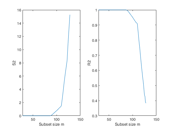
    %The forward plot of s2 shows that initially the estimate is virtually
    %zero. The four line segments comprising the plot correspond to the four
    %groups of observations
    % Plot of the monitoring of S2 and R2
    figure;
    subplot(1,2,1)
    plot(S2(:,1),S2(:,2))
    xlabel('Subset size m');
    ylabel('S2');
    subplot(1,2,2)
    plot(S2(:,1),S2(:,3))
    xlabel('Subset size m');
    ylabel('R2');
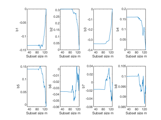
    %The forward plots of the estimates of the beta coefficients show that they are virtually constant until m = 86, after which they start fluctuating in different directions.
    % Plots of the monitoring of "Estimates of beta coefficients"
    figure;
    for j=3:size(Bols,2)
    subplot(2,4,j-2)
    plot(Bols(:,1),Bols(:,j))
    xlabel('Subset size m');
    ylabel(['b' num2str(j-2)]);
    end
    end
    Total estimated time to complete LMS:  0.06 seconds 
    
    Click here for the graphical output of this example (link to Ro.S.A. website)

  • Store units forming subsets in selected steps.
  • In this example the units forming subset are stored just for selected steps.

    load('hawkins.txt');
    y=hawkins(:,9);
    X=hawkins(:,1:8);
    rng('default')
    rng(100)
    [out]=LXS(y,X,'nsamp',10000);
    [mdr,Un,BB,Bols,S2] = FSRmdr(y,X,out.bs,'bsbsteps',[30 60]);
    if isnan(S2)
    disp('NoFullRank in initial subset, please rerun FSRmdr')
    else
    % BB has just two columns
    % First column contains information about units forming subset at step m=30
    % sum(~isnan(BB(:,1))) is 30
    % Second column contains information about units forming subset at step m=60
    % sum(~isnan(BB(:,2))) is 60
    disp(sum(~isnan(BB(:,1))))
    disp(sum(~isnan(BB(:,2))))
    end
    Total estimated time to complete LMS:  0.05 seconds 
        30
    
        60


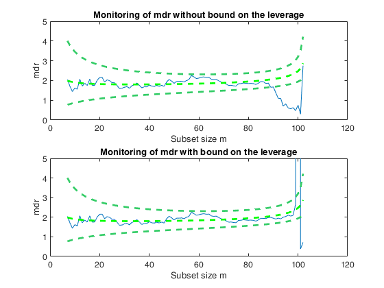
  • Example of the use of option threshlevoutX.
  • In this example a set of remote units is added to a cloud of points.

    % The purpose of this example is to show that in presence of units very far
    % from the bulk of th data (bad or good elverage points) it is necessary to
    % bound their effect putting a constraint on their leverage hi=xi'(X'X)xi
    rng(10000)
    n=100;
    p=1;
    X=randn(n,p);
    epsil=10;
    beta=ones(p,1);
    y=X*beta+randn(n,1)*epsil;
    % Add 10 very remote points
    add=3;
    Xadd=X(1:add,:)+5000;
    yadd=y(1:add)+200;
    Xall=[X;Xadd];
    yall=[y;yadd];
    outLXS=LXS(y,X);
    bs=outLXS.bs;
    subplot(2,1,1)
    out1=FSRmdr(yall,Xall,bs,'plots',1);
    xylim=axis;
    ylabel('mdr')
    title('Monitoring of mdr without bound on the leverage')
    subplot(2,1,2)
    out2=FSRmdr(yall,Xall,bs,'plots',1,'threshlevoutX',10);
    ylim(xylim(3:4));
    ylabel('mdr')
    title('Monitoring of mdr with bound on the leverage')
    Total estimated time to complete LMS:  0.01 seconds 
    Warning: Upper limit of y axis of the mdr forward plot set to 20 
    
    Click here for the graphical output of this example (link to Ro.S.A. website)

    Input Arguments

    expand all

    y — Response variable. Vector.

    Response variable, specified as a vector of length n, where n is the number of observations. Each entry in y is the response for the corresponding row of X.

    Missing values (NaN's) and infinite values (Inf's) are allowed, since observations (rows) with missing or infinite values will automatically be excluded from the computations.

    Data Types: single| double

    X — Predictor variables. Matrix.

    Matrix of explanatory variables (also called 'regressors') of dimension n x (p-1) where p denotes the number of explanatory variables including the intercept.

    Rows of X represent observations, and columns represent variables. By default, there is a constant term in the model, unless you explicitly remove it using input option intercept, so do not include a column of 1s in X. Missing values (NaN's) and infinite values (Inf's) are allowed, since observations (rows) with missing or infinite values will automatically be excluded from the computations.

    Data Types: single| double

    bsb — list of units forming the initial subset. Vector.

    If bsb=0 (default) then the procedure starts with p units randomly chosen else if bsb is not 0 the search will start with m0=length(bsb)

    Data Types: single| double

    Name-Value Pair Arguments

    Specify optional comma-separated pairs of Name,Value arguments. Name is the argument name and Value is the corresponding value. Name must appear inside single quotes (' '). You can specify several name and value pair arguments in any order as Name1,Value1,...,NameN,ValueN.

    Example: 'bsbmfullrank',1 , 'init',100 starts monitoring from step m=100 , 'intercept',false , 'internationaltrade',true , 'msg',1 , 'nocheck',true , 'threshlevoutX',5 , 'plots',1

    bsbmfullrank —What to do in case subset at step m (say bsbm) produces a non singular X.scalar.

    This options controls what to do when rank(X(bsbm,:)) is smaller then number of explanatory variables.

    If bsbmfullrank = 1 (default is 1) these units (whose number is say mnofullrank) are constrained to enter the search in the final n-mnofullrank steps else the search continues using as estimate of beta at step m the estimate of beta found in the previous step.

    Example: 'bsbmfullrank',1

    Data Types: double

    bsbsteps —Save the units forming subsets.vector.

    It specifies for which steps of the fwd search it is necessary to save the units forming subsets. If bsbsteps is 0 we store the units forming subset in all steps. If bsbsteps=[] or omitted, the default is to store the units forming subset in all steps if n<=5000, else to store the units forming subset at steps init and steps which are multiple of 100. For example, as default, if n=753 and init=6, units forming subset are stored for m=init, 100, 200, 300, 400, 500 and 600.

    Example: 'bsbsteps',[100 200] stores the unis forming subset in steps 100 and 200.

    Data Types: double

    constr —Constrained search.vector.

    r x 1 vector which contains the list of units which are forced to join the search in the last r steps. The default is constr=[].

    No constraint is imposed

    Example: 'constr',[1:10] forces the first 10 units to join the subset in the last 10 steps

    Data Types: double

    init —Search initialization.scalar.

    It specifies the point where to initialize the search and start monitoring required diagnostics. If it is not specified it is set equal to: p+1, if the sample size is smaller than 40;

    min(3*p+1,floor(0.5*(n+p+1))), otherwise.

    Example: 'init',100 starts monitoring from step m=100

    Data Types: double

    intercept —Indicator for constant term.true (default) | false.

    Indicator for the constant term (intercept) in the fit, specified as the comma-separated pair consisting of 'Intercept' and either true to include or false to remove the constant term from the model.

    Example: 'intercept',false

    Data Types: boolean

    internationaltrade —criterion for updating subset.boolean.

    If internationaltrade is true (default is false) residuals which have large of the final column of X (generally quantity) are reduced. Note that this guarantees that leverge units which have a large value of X will tend to stay in the subset. This option is particularly useful in the context of international trade data where we regress value (value=price*Q) on quantity (Q). In other words, we use the residuals as if we were regressing y/X (that is price) on the vector of ones.

    Example: 'internationaltrade',true

    Data Types: boolean

    msg —Level of output to display.scalar.

    It controls whether to display or not messages about great interchange on the screen If msg==1 (default) messages are displayed on the screen else no message is displayed on the screen

    Example: 'msg',1

    Data Types: double

    nocheck —Check input arguments.boolean.

    If nocheck is equal to true no check is performed on matrix y and matrix X. Notice that y and X are left unchanged. In other words the additioanl column of ones for the intercept is not added. As default nocheck=false. The controls on h, alpha and nsamp still remain

    Example: 'nocheck',true

    Data Types: boolean

    threshlevoutX —threshold for high leverage units.scalar | empty value.

    Threshold to bound the effect of high leverage units in the computation of deletion residuals. In the computation of the quantity $h_i(m^*) = x_i^T\{X(m^*)^TX(m^*)\}^{-1}x_i$, $i \notin S^{(m)}_*$, units which very far from the bulk of the data (represented by $X(m^*)$) will have a huge value of $h_i(m^*)$ and consequently of the deletion residuals.

    In order to tackle this problem it is possible to put a bound to the value of $h_i(m^*)$. For example threshlevoutX=r imposes the contrainst that $h_i(m^*)$ cannot exceed $r \times p/m$. The default value of threshlevoutX is empty, which means that no threshold is imposed.

    Example: 'threshlevoutX',5

    Data Types: double

    plots —Plot on the screen.scalar.

    If equal to one a plot of minimum deletion residual appears on the screen with 1%, 50% and 99% confidence bands else (default) no plot is shown.

    Remark: the plot which is produced is very simple. In order to control a series of options in this plot and in order to connect it dynamically to the other forward plots it is necessary to use function mdrplot.

    Example: 'plots',1

    Data Types: double

    Output Arguments

    expand all

    mdr —Monitoring of minimum deletion residual at each step of the forward search. n -init -by- 2 matrix

    1st col = fwd search index (from init to n-1).

    2nd col = minimum deletion residual.

    REMARK: if in a certain step of the search matrix is singular, this procedure checks how many observations produce a singular matrix. In this case mdr is a column vector which contains the list of units for which matrix X is non singular.

    Un —Units included in each step. Matrix

    (n-init) x 11 Matrix which contains the unit(s) included in the subset at each step of the search.

    REMARK: in every step the new subset is compared with the old subset. Un contains the unit(s) present in the new subset but not in the old one.

    Un(1,2) for example contains the unit included in step init+1.

    Un(end,2) contains the units included in the final step of the search.

    BB —Units belonging to subset in each step. Matrix

    n x (n-init+1) or n-by-length(bsbsteps) matrix (depending on input option bsbsteps) which contains information about the units belonging to the subset at each step of the forward search.

    BB has the following structure 1-st row has number 1 in correspondence of the steps in which unit 1 is included inside subset and a missing value for the other steps ......

    (n-1)-th row has number n-1 in correspondence of the steps in which unit n-1 is included inside subset and a missing value for the other steps n-th row has number n in correspondence of the steps in which unit n is included inside subset and a missing value for the other steps The size of matrix BB is n x (n-init+1) if option input bsbsteps is 0 else the size is n-by-length(bsbsteps).

    Bols —OLS coefficents. Matrix

    (n-init+1) x (p+1) matrix containing the monitoring of estimated beta coefficients in each step of the forward search.

    S2 —S2 and R2. Matrix

    (n-init+1) x 3 matrix containing the monitoring of S2 (2nd column)and R2 (third column) in each step of the forward search.

    More About

    expand all

    Additional Details

    Let $S^{(m)}_* \in \cal{M}$ be the optimum subset of size $m$, for which the matrix of regressors is $X(m^*)$. Least squares applied to this subset yields parameter estimates $\hat{\beta}(m^*)$ and $s^2(m^*)$, the mean square estimate of $\sigma^2$ on $m-p$ degrees of freedom. Residuals can be calculated for all observations including those not in $S^{(m)}_*$. The $n$ resulting least squares residuals are \begin{equation} e_i(m^*) = y_i -x_i^T\hat{\beta}(m^*). \label{eq2.14a} \end{equation} The search moves forward with the subset $S^{(m+1)}_*$ consisting of the observations with the $m+1$ smallest absolute values of $e_i(m^*)$. When $m < n$ the estimates of the parameters are based on only those observations giving the central $m$ residuals.

    To test for outliers the deletion residual is calculated for the $n-m$ observations not in $S^{(m)}_*$. These residuals are \begin{equation} r_i^*(m^*) = \frac{y_{i} - x_{i}^T\hat{\beta}(m^*)} { \sqrt{s^2(m^*)\{1 + h_i(m^*)\}}} = \frac{e_{i}(m^*)} { \sqrt{s^2(m^*)\{1 + h_i(m^*)\}}}, \end{equation} where $h_i(m^*) = x_i^T\{X(m^*)^TX(m^*)\}^{-1}x_i$; the leverage of each observation depends on $S^{(m)}_*$. Let the observation nearest to those constituting $S^{(m)}_*$ be $i_{\mbox{min}}$ where

    \[ i_{\mbox{min}} = \arg \min | r^*_i(m^*)| \; \mbox{for} \; i \notin S^{(m)}_*, \]

    the observation with the minimum absolute deletion residual among those not in $S^{(m)}_*$. This function computes $r_i^*(m^*)$ for $m^*=init, init+1, \ldots, n-1$.

    References

    Atkinson, A.C. and Riani, M. (2000), "Robust Diagnostic Regression Analysis", Springer Verlag, New York.

    Atkinson, A.C. and Riani, M. (2006), Distribution theory and simulations for tests of outliers in regression, "Journal of Computational and Graphical Statistics", Vol. 15, pp. 460-476.

    Riani, M. and Atkinson, A.C. (2007), Fast calibrations of the forward search for testing multiple outliers in regression, "Advances in Data Analysis and Classification", Vol. 1, pp. 123-141.

    See Also

    |

    This page has been automatically generated by our routine publishFS