tclustregeda
tclustregeda performs robust linear grouping analysis for a series of values of the trimming factor
Syntax
Description
tclustregeda performs tclustreg for a series of values of the trimming factor alpha, for given k (number of groups), restrfactor (restriction factor) and alphaX (second level trimming or cluster weighted model).
In order to increase the speed of the computations, parfor is used.
tclustregeda of contaminated X data using all default options.out
=tclustregeda(y,
X,
k,
restrfact,
alphaLik,
alphaX)
Examples
tclustregeda of contaminated X data using all default options.
The X data have been introduced by Gordaliza, Garcia-Escudero and Mayo-Iscar (2013).
% The dataset presents two parallel components without contamination.
X  = load('X.txt');
y = X(:,end);
X =X(:,1:end-1);
% Contaminate the first 4 units
y(1:4)=y(1:4)+6;
% Use 2 groups
k = 2 ;
% Set restriction factor
restrfact = 5;
% Value of trimming
alphaLik = 0.10:-0.01:0;
% cwm
alphaX = 1;
out = tclustregeda(y,X,k,restrfact,alphaLik,alphaX);
 tclustregeda with a noise variable and personalized plots.
tclustregeda with a noise variable and personalized plots.Use the X data of the previous example.
% set(0,'DefaultFigureWindowStyle','docked')
X = load('X.txt');
y = X(:,end);
rng(100)
X = [randn(length(y),1) X(:,1:end-1)];
% Contaminate the first 4 units
y(1:4)=y(1:4)+6;
% Use 2 groups
k = 2 ;
restrfact = 5;
% Value of trimming
alphaLik = [0.10 0.06 0.03 0];
% cwm
alphaX = 1;
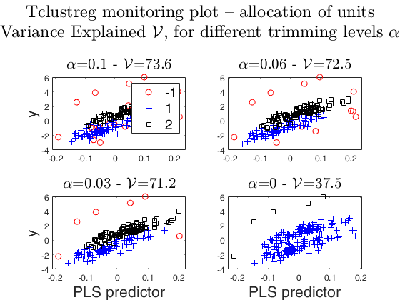
% Personalize plots. Just show the gscatter plot. In this case given
% that there is more than one explanatory variable PLS regression
% (adding the dummies for the classified units) is performed. In the
% gscatter plots the percentage of variance explained by the first
% linear combination of the X variables is given in the title of each
% panel of the gscatter plot.
plots=struct;
plots.name={'gscatter'};
out = tclustregeda(y,X,k,restrfact,alphaLik,alphaX,'plots',plots);
ClaLik with untrimmed units selected using crisp criterion
100%[===================================================]
tclustregeda: example with multiple explanatory variables, with yXplot.
X  = load('X.txt');
y = X(:,end);
rng(100)
X = [randn(length(y),4) X(:,1:end-1)];
k=2;
alphaLik = [0.10:-0.01:0]' ;
alphaX = 0;
restrfact =1;
mixt=2;
plots=struct;
% plots.name={'gscatter','postprob'};
% plots.alphasel=[0.05 0.03 0];
plots.name={'all'};
% 'UnitsSameGroup',152,
out = tclustregeda(y,X,k,restrfact,alphaLik,alphaX,'mixt',2,'msg',0,'plots',plots);
Input Arguments
y — Response variable.
Vector.
A vector with n elements that contains the response variable.
y can be either a row or a column vector.
Data Types: single|double
X — Explanatory variables (also called 'regressors').
Matrix.
Data matrix of dimension . Rows of X represent observations, and columns represent variables. Missing values (NaN's) and infinite values (Inf's) are allowed, since observations (rows) with missing or infinite values will automatically be excluded from the computations.
Data Types: single|double
k — Number of clusters.
Scalar.
This is a guess on the number of data groups.
Data Types: single|double
restrfact — restriction factor for regression residuals and covariance
matrices of the explanatory variables.
Scalar or vector with two
elements.
If restrfact is a scalar it controls the differences among group scatters of the residuals. The value 1 is the strongest restriction. If restrfactor is a vector with two elements the first element controls the differences among group scatters of the residuals and the second the differences among covariance matrices of the explanatory variables. Note that restrfactor(2) is used just if input option alphaX=1, that is if constrained weighted model for X is assumed.
Data Types: single|double
alphaLik — trimming level to monitor.
Vector.
Vector which specifies the values of trimming levels which have to be considered.
alpha is a vector which contains decreasing elements which lie in the interval 0 and 0.5.
For example if alpha=[0.1 0.05 0] tclustregeda considers these 3 values of trimming level.
If alphaLik=0 tclustregeda does not trim. The default for alphaLik is vector [0.1 0.05 0]. The sequence is forced to be monotonically decreasing.
Data Types: single| double
alphaX — Second-level trimming or constrained weighted model for X.
Scalar.
alphaX is a value in the interval [0 1].
- If alphaX=0 there is no second-level trimming.
- If alphaX is in the interval [0 0.5] it indicates the fixed proportion of units subject to second level trimming.
In this case alphaX is usually smaller than alphaLik.
For further details see Garcia-Escudero et. al. (2010).
- If alphaX is in the interval (0.5 1), it indicates a Bonferronized confidence level to be used to identify the units subject to second level trimming. In this case the proportion of units subject to second level trimming is not fixed a priori, but is determined adaptively.
For further details see Torti et al. (2018).
- If alphaX=1, constrained weighted model for X is assumed (Gershenfeld, 1997). The CWM estimator is able to take into account different distributions for the explanatory variables across groups, so overcoming an intrinsic limitation of mixtures of regression, because they are implicitly assumed equally distributed. Note that if alphaX=1 it is also possible to apply using restrfactor(2) the constraints on the cov matrices of the explanatory variables.
For further details about CWM see Garcia-Escudero et al.
(2017) or Torti et al. (2018).
Data Types: single|double
Name-Value Pair Arguments
Specify optional comma-separated pairs of Name,Value arguments.
Name is the argument name and Value
is the corresponding value. Name must appear
inside single quotes (' ').
You can specify several name and value pair arguments in any order as
Name1,Value1,...,NameN,ValueN.
 'intercept',1
, 'mixt',1
, 'equalweights',true
, 'nsamp',1000
, 'refsteps',15
, 'reftol',1e-05
, 'commonslope',true
, 'plots', 1
, 'msg',1
, 'nocheck',1
, 'RandNumbForNini',''
, 'UnitsSameGroup',[20 34]
, 'numpool',4
, 'cleanpool',true
, 'we',[0.2 0.2 0.2 0.2 0.2]
intercept
—Indicator for constant term.scalar.
If 1, a model with constant term will be fitted (default), else no constant term will be included.
Example: 'intercept',1
Data Types: double
mixt
—mixture modelling or crisp assignment.scalar.
Option mixt specifies whether mixture modelling or crisp assignment approach to model based clustering must be used.
In the case of mixture modelling parameter mixt also controls which is the criterior to find the untrimmed units in each step of the maximization If mixt >=1 mixture modelling is assumed else crisp assignment.
In mixture modelling the likelihood is given by
\prod_{i=1}^n \sum_{j=1}^k \pi_j \phi (y_i \; x_i' , \beta_j , \sigma_j), while in crisp assignment the likelihood is given by \prod_{j=1}^k \prod _{i\in R_j} \pi_j \phi (y_i \; x_i' , \beta_j , \sigma_j),where R_j contains the indexes of the observations which are assigned to group j, Remark - if mixt>=1 previous parameter equalweights is automatically set to 1.
Parameter mixt also controls the criterion to select the units to trim if mixt == 2 the h units are those which give the largest contribution to the likelihood that is the h largest values of
\sum_{j=1}^k \pi_j \phi (y_i \; x_i' , \beta_j , \sigma_j) \qquad i=1, 2, ..., n elseif mixt==1 the criterion to select the h units is exactly the same as the one which is used in crisp assignment. That is: the n units are allocated to a cluster according to criterion \max_{j=1, \ldots, k} \hat \pi'_j \phi (y_i \; x_i' , \beta_j , \sigma_j)and then these n numbers are ordered and the units associated with the largest h numbers are untrimmed.
Example: 'mixt',1
Data Types: single | double
equalweights
—cluster weights in the concentration and assignment steps.logical.
A logical value specifying whether cluster weights shall be considered in the concentration, assignment steps and computation of the likelihood.
if equalweights = true we are (ideally) assuming equally sized groups by maximizing the likelihood. Default value false.
Example: 'equalweights',true
Data Types: Logical
nsamp
—number of subsamples to extract.scalar | matrix with k*p columns.
If nsamp is a scalar it contains the number of subsamples which will be extracted.
If nsamp=0 all subsets will be extracted.
If the number of all possible subset is <300 the default is to extract all subsets, otherwise just 300.
If nsamp is a matrix it contains in the rows the indexes of the subsets which have to be extracted. nsamp in this case can be conveniently generated by function subsets.
nsamp must have k*p columns. The first p columns are used to estimate the regression coefficient of group 1... the last p columns are used to estimate the regression coefficient of group k.
Example: 'nsamp',1000
Data Types: double
refsteps
—Number of refining iterations.scalar.
Number of refining iterations in each subsample. Default is 10.
refsteps = 0 means "raw-subsampling" without iterations.
Example: 'refsteps',15
Data Types: single | double
reftol
—Tolerance for the refining steps.scalar.
The default value is 1e-14;
Example: 'reftol',1e-05
Data Types: single | double
commonslope
—Impose constraint of common slope regression coefficients.boolean.
If commonslope is true, the groups are forced to have the same regression coefficients (apart from the intercepts).
The default value of commonslope is false;
Example: 'commonslope',true
Data Types: boolean
plots
—Plot on the screen.scalar structure.
Case 1: plots option used as scalar.
- If plots=0, plots are not generated.
- If plots=1 (default), 6 plots are shown on the screen.
The first plot ("monitor") shows 4 or 6 panels monitoring between two consecutive values of alpha the change in classification using ARI index (top left panel), the relative change in beta (top right panel) ($||\beta_{\alpha_1}-\beta_{\alpha_2}||^2/||\beta_{\alpha_2}||^2 the relative change in \sigma^2 (third panel) the relative change in \sigma^2 corrected (fourth panel) and if alphaX=1, the relative change in centroids (fifth panel), the relative change in covariance matrices using squared euclidean distance (sixth panel).
The second plot ("UnitsTrmOrChgCla") is a bsb plot which shows the monitoring of the units which changed classification (shown in red) or were trimmed at least once.
The third plot shows ("PostProb") is a 4 panel parallel coordinate plots which shows the monitoring of posterior probabilities. Four versions of parallel coordinateds plots are proposed. The first two use function parallelcoords and refer respectively to all the units (left panel) or the units which were trimmed or changed allocation (right panels). The two bottom panels are exactly equal as top panels but use function parallelplot.
The fourth plot ("PostProb") is 4 panel parallel coordinate plots which shows the monitoring of posterior probabilities. Four versions of parallel coordinateds plots are proposed. The first two use function parallelcoords and refer respectively to all the units (left panel) or the units which were trimmed or changed allocation (right panels). The two bottom panels are exactly equal as top panels but use function parallelplot.
The fifth plot is a scatter of y versus X (or a yXplot in case X ha more than one column) with all the regression lines for each value of alphaLik shown. Units trimmed are shown in correspondence of max(alphaLik).
The sixth plot ("gscatter plot") shows a series of subplots which monitor the classification for each value of alpha. In order to make sure that consistent labels are used for the groups, between two consecutive values of alpha, we assign label r to a group if this group shows the smallest distance with group r for the previous value of alpha. The type of plot which is used to monitor the stability of the classification depends on the value of p (number of explanatory variables excluding the intercept).
* for p=0, we use histograms of the univariate data (function histFS is called).
* for p=1, we use the scatter plot of y against the unique explanatory variable (function gscatter is called).
* for p>=2, we use partial least square regression (see function plsregress) and use the scatter plot of y against the predictor scores Xs, that is, the first PLS component that is linear combination of the variables in X.
Case 2: plots option used as struct.
If plots is a structure it may contain the following fields:
| Value | Description |
|---|---|
name |
cell array of strings which enables to specify which plot to display. plots.name={'monitor'; 'UnitsTrmOrChgCla'; 'PostProb'; 'Sigma';... 'ScatterWithRegLines'; 'gscatter'}; is exactly equivalent to plots=1 For the explanation of the above plots see plots=1. If plots.name=={ 'monitor'; 'UnitsTrmOrChgCla'; 'PostProb'; 'Sigma';... 'ScatterWithRegLines'; 'gscatter'; ... 'Beta';'Siz'}; or plots.name={'all'}; it is also possible to monitor the beta coefficients for each group ('Beta') and the size of the groups (Siz). Note that the trajectories of beta coefficients are standardized in order to have all of them on a comparable scale. |
alphasel |
numeric vector which speciies for which values of alpha it is possible to see the classification (in plot gscatter) or the superimposition of regression lines (in plot ScatterWithRegLines) . For example if plots.alphasel =[ 0.05 0.02], the classification in plot gscatter and the regression lines in plot ScatterWithRegLines will be shown just for alphaLik=0.05 and alphaLik=0.02; If this field is not specified plots.alphasel=alphaLik and therefore the classification is shown for each value of alphaLik. |
Example: 'plots', 1
Data Types: single | double | struct
msg
—Level of output to display.scalar.
Scalar which controls whether to display or not messages on the screen.
If msg=0 nothing is displayed on the screen.
If msg=1 (default) messages are displayed on the screen about estimated time to compute the estimator or the number of subsets in which there was no convergence.
If msg=2 detailed messages are displayed. For example the information at iteration level.
Example: 'msg',1
Data Types: single | double
nocheck
—Check input arguments.scalar.
If nocheck is equal to 1 no check is performed on vector y and matrix X.
As default nocheck=0.
Example: 'nocheck',1
Data Types: single | double
RandNumbForNini
—Pre-extracted random numbers to initialize proportions.matrix.
Matrix with size k-by-size(nsamp,1) containing the random numbers which are used to initialize the proportions of the groups. This option is effective just if nsamp is a matrix which contains pre-extracted subsamples. The purpose of this option is to enable the user to replicate the results in case routine tclust is called using a parfor instruction (as it happens for example in routine IC, where tclust is called through a parfor for different values of the restriction factor).
The default value of RandNumbForNini is empty that is random numbers from uniform are used.
Example: 'RandNumbForNini',''
Data Types: single | double
UnitsSameGroup
—list of the units which must (whenever possible)
have a particular label.numeric vector.
For example if UnitsSameGroup=[20 26], means that group which contains unit 20 is always labelled with number 1. Similarly, the group which contains unit 26 is always labelled with number 2, (unless it is found that unit 26 already belongs to group 1). In general, group which contains unit UnitsSameGroup(r) where r=2, ...length(kk)-1 is labelled with number r (unless it is found that unit UnitsSameGroup(r) has already been assigned to groups 1, 2, ..., r-1).
Example: 'UnitsSameGroup',[20 34]
Data Types: integer vector
numpool
—The number of parallel sessions to open.integer.
If numpool is not defined, then it is set equal to the number of physical cores in the computer.
Example: 'numpool',4
Data Types: integer vector
cleanpool
—Function name.scalar {0,1}.
Indicated if the open pool must be closed or not. It is useful to leave it open if there are subsequent parallel sessions to execute, so that to save the time required to open a new pool.
Example: 'cleanpool',true
Data Types: integer | logical
we
—Vector of observation weights.vector.
A vector of size n-by-1 containing application-specific weights that the user needs to apply to each observation. Default value is a vector of ones.
Example: 'we',[0.2 0.2 0.2 0.2 0.2]
Data Types: double
Output Arguments
out — description
Structure
Structure which contains the following fields
| Value | Description |
|---|---|
IDX |
n-by-length(alphaLik) matrix containing assignment of each unit to each of the k groups. Cluster names are integer numbers from 1 to k: -1 indicates first level trimmed observations; -2 indicates second level trimmed observations. observations. First column refers of out.IDX refers to alphaLik(1), second column of out.IDX refers to alphaLik(2), ..., last column refers to alphaLik(end). |
Beta |
3D array of size k-by-p-by-length(alphaLik) containing the monitoring of the regression coefficients for each value of alphaLik. out.Beta(:,:,1), refers to alphaLik(1) ..., out.Beta(:,:,end) refers to alphaLik(end). First row in each slice refers to group 1, second row refers to group 2 ... |
Sigma2y |
matrix of size k-by-length(alphaLik) containing in column j, with j=1, 2, ..., length(alphaLik), the estimates of the k (constrained) variances of the regressions lines (hyperplanes) associated with alphaLik(j). |
Sigma2yc |
matrix of size k-by-length(alphaLik) containing in column j, with j=1, 2, ..., length(alphaLik), the estimates of the k (constrained) unbiased variances of the regressions lines (hyperplanes) associated with alphaLik(j). In order to make the estimates of sigmas unbiased we apply Tallis correction factor. |
Nopt |
matrix of size k-by-length(alphaLik) containing in column j, with j=1, 2, ..., length(alphaLik), the sizes of the of the k groups. |
Vopt |
column vector of length(alphaLik) containing the value of the target likelihod for each value of alphaLik. |
Amon |
Amon stands for alphaLik monitoring. Matrix of size (length(alphaLik)-1)-by-7 which contains for two consecutive values of alpha the monitoring of six quantities (change in classification, change in betas, sigmas, correted sigmas and if cwm also centroid and coariance in the X space. 1st col = value of alphaLik. 2nd col = ARI index. 3rd col = relative squared Euclidean distance between two consecutive beta. 4th col = relative squared Euclidean distance between two consecutive vectors of variances of the errors of the k regressions. 5th col = relative squared Euclidean distance between two consecutive vectors of correct variances of the errors of the k regressions. 6th col = relative squared Euclidean distance between two consecutive \hat \mu_X. 7th col = relative squared Euclidean distance between two consecutive \hat \Sigma_X. |
MU |
3D array of size k-by-(p-1)-by-length(alphaLik) containing the monitoring of the X centroids for each value of alphaLik. out.MU(:,:,1), refers to alphaLik(1) ..., out.MU(:,:,end) refers to alphaLik(end). First row in each slice refers to group 1, second row refers to group 2 ... This field is present only if input option alphaX is 1. |
SIGMA |
cell of length length(alphaLik) containing in element j, with j=1, 2, ..., length(alphaLik), the 3D array of size (p-1)-by-(p-1)-by-k containing the k (constrained) estimated covariance matrices of X associated with alphaLik(j). This field is present only if input option alphaX is 1. |
UnitsTrmOrChgCla |
Matrix containing information about the units (n1) which were trimmed or changed classification at least once in the forward search. The size of out.UnitsTrmOrChgCla is n1-by-length(alphaLik)+1; 1st col = list of the units which were trimmed or changed classification at least once. 2nd col = allocation of the n1 units in step alphaLik(1) 3rd col = allocation of the n1 units in step alphaLik(2) ... last col = allocation of the n1 units in step alphaLik(end) |
Postprob |
Posterior probabilities. 3D array of size n-by-k-length(alphaLik) containing the monitoring of posterior probabilities. |
units |
structure containing the following fields: units.UnitsTrmOrChgCla=units trimmed at least onece or changed classification at least once. units.UnitsChgCla=units which changed classification at least once (i.e. from group 1 to group 3 ...). units.UnitsTrm=units trimmed at least once. units.UnitsNeverAssigned=units never assigned (i.e. all those which have always been trimmed by first level or second level). |
varargout —In jth
position the structure which comes out from procedure
tclustreg applied to alphaLik(j), with j =1, 2, .
outcell : cell of length length(alpha)
.., length(alphaLik).
More About
Additional Details
This procedure extends to tclustreg the so-called monitoring approach.
The philosophy is to investigate how the results change as the trimming proportion alpha reduces. This function enables us to monitor the change in classification (measured by the ARI index) and the change in regression coefficients and error variances (measured by the relative squared Euclidean distances).
Note that there is a non-identifiability of a finite mixture distribution caused by the invariance of the mixture density function to components relabeling. In order to make sure that consistent labels are used for the groups, between two consecutive values of alpha, we call we assign label r to a group if this group shows the smallest distance with group r for the previous value of alpha.
More precisely, once the labelling is fixed for the largest value of the trimming factor supplied, if \alpha_r and \alpha_s denote two consecutive levels of trimming (\alpha_r>\alpha_s) and \beta_{j,\alpha_r} given \beta_{j,\alpha_r} In order to be consistent along the different runs it is possible to specify through option UnitsSameGroup the list of the units which must (whenever possible) have a particular label.
References
Garcia-Escudero, L.A., Gordaliza A., Greselin F., Ingrassia S., and Mayo-Iscar A. (2016), The joint role of trimming and constraints in robust estimation for mixtures of gaussian factor analyzers, "Computational Statistics & Data Analysis", Vol. 99, pp. 131-147.
Garcia-Escudero, L.A., Gordaliza, A., Greselin, F., Ingrassia, S. and Mayo-Iscar, A. (2017), Robust estimation of mixtures of regressions with random covariates, via trimming and constraints, "Statistics and Computing", Vol. 27, pp. 377-402.
Garcia-Escudero, L.A., Gordaliza A., Mayo-Iscar A., and San Martin R. (2010), Robust clusterwise linear regression through trimming, "Computational Statistics and Data Analysis", Vol. 54, pp.3057-3069.
Cerioli, A. and Perrotta, D. (2014). Robust Clustering Around Regression Lines with High Density Regions. Advances in Data Analysis and Classification, Vol. 8, pp. 5-26.
Torti F., Perrotta D., Riani, M. and Cerioli A. (2019). Assessing Robust Methodologies for Clustering Linear Regression Data, "Advances in Data Analysis and Classification", Vol. 13, pp. 227–257, https://doi.org/10.1007/s11634-018-0331-4