
|
tclusteda |
tclustICgpcm |
 |
tclustIC
tclustIC computes tclust for different number of groups k and restriction factors c
Description
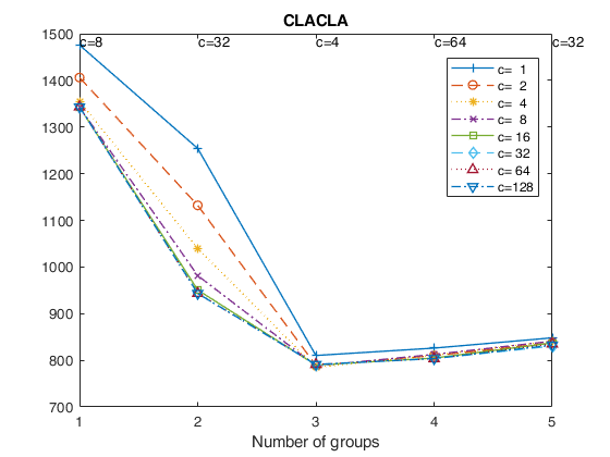
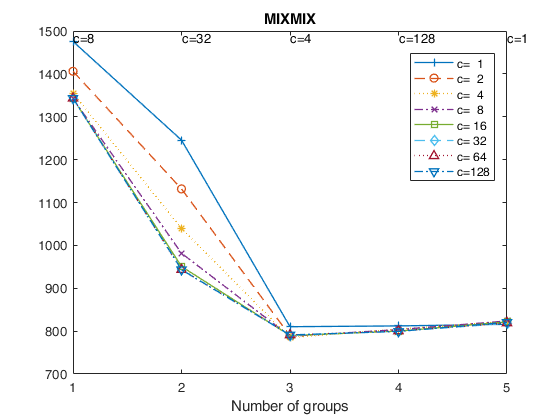
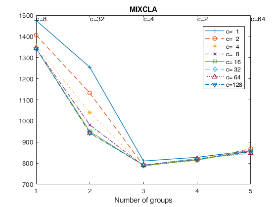
tclustIC (where the last two letters stand for 'Information Criterion') computes the values of BIC (MIXMIX), ICL (MIXCLA) or CLA (CLACLA), for different values of k (number of groups) and different values of c (restriction factor), for a prespecified level of trimming. If Parallel Computing toolbox is installed, parfor is used to compute tclust for different values of c. In order to minimize randomness, given k, the same subsets are used for each value of c.
Automatic choice of k in an example with 3 components and prefixed overlap.out
=tclustIC(Y,
Name, Value)
Examples
 Automatic choice of k for geyser data using alpha=0.1.
Automatic choice of k for geyser data using alpha=0.1.
Y=load('geyser2.txt');
out=tclustIC(Y,'cleanpool',false,'plots',1,'alpha',0.1);
% Write out.MIXMIX as MATLAB table
disp('MIXMIX (BIC)')
if verLessThan ('matlab','8.2.0');
VariableNames={'c_1'; 'c_2'; 'c_4'; 'c_8'; 'c_16'; 'c_32'; 'c_64'; 'c_128'};
disp(VariableNames')
disp(out.MIXMIX)
disp('Rows refers to k (number of groups')
else
RowNames=cellstr([repmat('k=',length(out.kk),1) num2str(out.kk')]);
VariableNames=matlab.lang.makeValidName(cellstr([repmat('c=',length(out.cc),1) num2str(out.cc')]));
disp(array2table(out.MIXMIX,'VariableNames',VariableNames','RowNames',RowNames))
end
% Find smallest value inside the table and write the corresponding
% values of k (number of groups) and c (restriction factor)
[valmin,indk]=min(out.MIXMIX);
[minIC,indc]=min(valmin);
disp(['Smallest value of IC is ' num2str(minIC) ' and takes place for'])
disp(['k=' num2str(out.kk(indk(indc))) ' and  c=' num2str(out.cc(indc))]);
k=1
k=2
k=3
k=4
k=5
The labels of c in the top part of the plot denote the values of c for which IC is minimum
MIXMIX (BIC)
            c_1       c_2       c_4       c_8       c_16      c_32      c_64     c_128
           ______    ______    ______    ______    ______    ______    ______    ______

    k=1    1475.7    1406.1    1355.4    1342.4    1342.8      1343      1343    1343.1
    k=2    1245.5    1131.7    1039.6    981.55    950.67    943.08    943.25    943.38
    k=3    810.31    788.98    784.84    787.93    789.65    790.51    790.93    791.15
    k=4    812.15    800.45    804.79    803.63    800.02    799.67    800.16    799.26
    k=5    815.93    819.29    822.69    823.62    821.51    818.13    818.99    820.41

Smallest value of IC is 784.8427 and takes place for
k=3 and  c=4
Automatic choice of k in an example with 3 components and prefixed overlap.
restrfact=5;
rng('default') % Reinitialize the random number generator to its startup configuration
rng(20000);
ktrue=3;
% n = number of observations
n=150;
% v= number of dimensions
v=2;
% Imposed average overlap
BarOmega=0.04;
out=MixSim(ktrue,v,'BarOmega',BarOmega, 'restrfactor',restrfact);
% data generation given centroids and cov matrices
[Y,id]=simdataset(n, out.Pi, out.Mu, out.S);
% Automatic choice of k
out=tclustIC(Y,'cleanpool',false,'plots',1,'nsamp',100);
% Plot of MIXMIX as function of c given k.
figure('units','normalized','outerposition',[0 0 1 1])
% Specify whether to use the same y scale for ALL plots
samescale=1;
kk=out.kk;
cc=out.cc;
lcc=length(cc);
IC=out.MIXMIX;
miny=min(min(IC));
maxy=max(max(IC));
seqcc=1:lcc;
for j=kk
subplot(1,length(kk),j)
hold('on')
plot(1:lcc,IC(j,:),'k')
[minICj,minICjind]=min(IC(j,:));
plot(seqcc(minICjind),minICj,'rs','MarkerSize',10)
xlim([1 length(cc)])
if samescale==1
ylim([miny maxy])
end
L = get(gca,'XLim');
set(gca,'XTick',linspace(L(1),L(2),lcc))
set(gca,'XTickLabel',num2str(cc'))
xlabel('Restr. fact. $c$','Interpreter','Latex')
title(['k=' num2str(j)])
end
suplabel('BIC (MIXMIX)','t');
Input Arguments
Y — Input data.
Matrix.
Data matrix containing n observations on v variables Rows of Y represent observations, and columns represent variables. Observations (rows) with missing (NaN) or or infinite (Inf) values will automatically be excluded from the computations.
Data Types: double
Name-Value Pair Arguments
Specify optional comma-separated pairs of Name,Value arguments.
Name is the argument name and Value
is the corresponding value. Name must appear
inside single quotes (' ').
You can specify several name and value pair arguments in any order as
Name1,Value1,...,NameN,ValueN.
 'kk',1:4
, 'cc',[1 2 4 8 128]
, 'whichIC','ALL'
, 'alpha',0
, 'nsamp',1000
, 'RandNumbForNini',''
, 'refsteps',10
, 'reftol',1e-05
, 'equalweights',true
, 'startv1',1
, 'restrtype','deter'
, 'plots',1
, 'numpool',4
, 'cleanpool',1
, 'msg',1
, 'nocheck',10
, 'Ysave',1
, 'UnitsSameGroup',[12 20]
, 'cshape',10
kk
—number of mixture components.integer vector.
Integer vector specifying the number of mixture components (clusters) for which the BIC is to be calculated.
Vector. The default value of kk is 1:5.
Example: 'kk',1:4
Data Types: int16 | int32 | single | double
cc
—values of restriction factor.vector.
A vector specifying the values of the restriction factor which have to be considered for the covariance matrices.
The default value of cc is [1 2 4 8 16 32 64 128]
Example: 'cc',[1 2 4 8 128]
Data Types: double
whichIC
—type of information criterion.character.
Character which specifies which information criteria must be computed for each k (number of groups) and each value of the restriction factor (c).
Possible values for whichIC are: 'MIXMIX' = a mixture model is fitted and to compute the information criterion the mixture likelihood is used. This option corresponds to the use of the Bayesian Information criterion (BIC). In output structure out just the matrix out.MIXMIX is given.
'MIXCLA' = a mixture model is fitted but to compute the information criterion the classification likelihood is used. This option corresponds to the use of the Integrated Complete Likelihood (ICL). In output structure out just the matrix out.MIXCLA is given.
'CLACLA' = everything is based on the classification likelihood. This information criterion will be called CLA. In output structure out just the matrix out.CLACLA is given.
'ALL' = both classification and mixture likelihood are used.
In this case all the three information criteria CLA, ICL and BIC are computed. In output structure out all the three matrices out.MIXMIX and out.MIXCLA and out.CLACLA are given.
Example: 'whichIC','ALL'
Data Types: character
alpha
—global trimming level.fraction | number of observations which have to be trimmed.
alpha is a scalar between 0 and 0.5 or an integer specifying the number of observations to be trimmed. If alpha = 0 all observations are considered.
More in detail, if 0 < alpha < 1 clustering is based on h = fix(n*(1-alpha)) observations. Else if alpha is an integer greater than 1 clustering is based on h=n-floor(alpha).
The default value of alpha which is used is 0.
Example: 'alpha',0
Data Types: single | double
nsamp
—number of subsamples to extract.scalar | matrix.
If nsamp is a scalar it contains the number of subsamples which will be extracted. If nsamp=0 all subsets will be extracted.
Remark - if the number of all possible subset is <300 the default is to extract all subsets, otherwise just 300.
- If nsamp is a matrix it contains in the rows the indexes of the subsets which have to be extracted. nsamp in this case can be conveniently generated by function subsets.
nsamp can have k columns or k*(v+1) columns. If nsamp has k columns the k initial centroids each iteration i are given by X(nsamp(i,:),:) and the covariance matrices are equal to the identity.
- If nsamp has k*(v+1) columns the initial centroids and covariance matrices in iteration i are computed as follows X1=X(nsamp(i,:),:) mean(X1(1:v+1,:)) contains the initial centroid for group 1 cov(X1(1:v+1,:)) contains the initial cov matrix for group 1 1 mean(X1(v+2:2*v+2,:)) contains the initial centroid for group 2 cov((v+2:2*v+2,:)) contains the initial cov matrix for group 2 1 ...
mean(X1((k-1)*v+1:k*(v+1))) contains the initial centroids for group k cov(X1((k-1)*v+1:k*(v+1))) contains the initial cov matrix for group k REMARK - if nsamp is not a scalar option option below startv1 is ignored. More precisely if nsamp has k columns startv1=0 elseif nsamp has k*(v+1) columns option startv1=1.
Example: 'nsamp',1000
Data Types: double
RandNumbForNini
—Pre-extracted random numbers to initialize proportions.matrix.
Matrix with size k-by-size(nsamp,1) containing the random numbers which are used to initialize the proportions of the groups. This option is effective just if nsamp is a matrix which contains pre-extracted subsamples and k is a scalar. The purpose of this option is to enable the user to replicate the results.
The default value of RandNumbForNini is empty, that is random numbers from uniform are used.
Example: 'RandNumbForNini',''
Data Types: single | double
refsteps
—Number of refining iterations.scalar.
Number of refining iterations in subsample. Default is 15. refsteps = 0 means "raw-subsampling" without iterations.
Example: 'refsteps',10
Data Types: single | double
reftol
—scalar.default value of tolerance for the refining steps.
The default value is 1e-14;
Example: 'reftol',1e-05
Data Types: single | double
equalweights
—cluster weights in the concentration and assignment steps.logical.
A logical value specifying whether cluster weights shall be considered in the concentration, assignment steps and computation of the likelihood. The default value is false.
Example: 'equalweights',true
Data Types: Logical
startv1
—how to initialize centroids and cov matrices.scalar.
If startv1 is 1 then initial centroids and and covariance matrices are based on (v+1) observations randomly chosen, else each centroid is initialized taking a random row of input data matrix and covariance matrices are initialized with identity matrices.
Remark 1- in order to start with a routine which is in the required parameter space, eigenvalue restrictions are immediately applied. The default value of startv1 is 1.
Remark 2 - option startv1 is used just if nsamp is a scalar (see for more details the help associated with nsamp).
Example: 'startv1',1
Data Types: single | double
restrtype
—type of restriction.character.
The type of restriction to be applied on the cluster scatter matrices. Valid values are 'eigen' (default), or 'deter'.
eigen implies restriction on the eigenvalues while deter implies restriction on the determinants. If restrtype is 'deter' it is possible to control the constraints on the shape matrices using optional input argument cshape.
Example: 'restrtype','deter'
Data Types: char
plots
—Plot on the screen.scalar.
If plots = 1, a plot of the BIC (MIXMIX), ICL (MIXCLA)curve and CLACLA is shown on the screen. The plots which are shown depend on the input option 'whichIC'.
Example: 'plots',1
Data Types: single | double
numpool
—number of pools for parellel computing.scalar.
If numpool > 1, the routine automatically checks if the Parallel Computing Toolbox is installed and distributes the random starts over numpool parallel processes. If numpool <= 1, the random starts are run sequentially. By default, numpool is set equal to the number of physical cores available in the CPU (this choice may be inconvenient if other applications are running concurrently). The same happens if the numpool value chosen by the user exceeds the available number of cores. REMARK 1: up to R2013b, there was a limitation on the maximum number of cores that could be addressed by the parallel processing toolbox (8 and, more recently, 12). From R2014a, it is possible to run a local cluster of more than 12 workers.
REMARK 2: Unless you adjust the cluster profile, the default maximum number of workers is the same as the number of computational (physical) cores on the machine.
REMARK 3: In modern computers the number of logical cores is larger than the number of physical cores. By default, MATLAB is not using all logical cores because, normally, hyper-threading is enabled and some cores are reserved to this feature.
REMARK 4: It is because of Remarks 3 that we have chosen as default value for numpool the number of physical cores rather than the number of logical ones. The user can increase the number of parallel pool workers allocated to the multiple start monitoring by: - setting the NumWorkers option in the local cluster profile settings to the number of logical cores (Remark 2). To do so go on the menu "Home|Parallel|Manage Cluster Profile" and set the desired "Number of workers to start on your local machine".
- setting numpool to the desired number of workers;
Therefore, *if a parallel pool is not already open*, UserOption numpool (if set) overwrites the number of workers set in the local/current profile. Similarly, the number of workers in the local/current profile overwrites default value of 'numpool' obtained as feature('numCores') (i.e. the number of physical cores).
Example: 'numpool',4
Data Types: double
cleanpool
—clean pool.scalar.
cleanpool is 1 if the parallel pool has to be cleaned after the execution of the routine. Otherwise it is 0. The default value of cleanpool is 1. Clearly this option has an effect just if previous option numpool is >
1.
Example: 'cleanpool',1
Data Types: single | double
msg
—Message on the screen.scalar.
Scalar which controls whether to display or not messages about code execution.
Example: 'msg',1
Data Types: single | double
nocheck
—Check input arguments.scalar.
If nocheck is equal to 1 no check is performed on matrix Y. As default nocheck=0.
Example: 'nocheck',10
Data Types: single | double
Ysave
—save input matrix.scalar.
Scalar that is set to 1 to request that the input matrix Y is saved into the output structure out. Default is 1, that is matrix Y is saved inside output structure out.
Example: 'Ysave',1
Data Types: single | double
UnitsSameGroup
—Units with same labels.numeric vector.
List of the units which must (whenever possible) have the same label. For example if UnitsSameGroup=[20 26], it means that group which contains unit 20 is always labelled with number 1. Similarly, the group which contains unit 26 is always labelled with number 2, (unless it is found that unit 26 already belongs to group 1). In general, group which contains unit UnitsSameGroup(r) where r=2, ...length(kk)-1 is labelled with number r (unless it is found that unit UnitsSameGroup(r) has already been assigned to groups 1, 2, ..., r-1). The default value of UnitsSameGroup is '' that is consistent labels are not imposed.
Example: 'UnitsSameGroup',[12 20]
Data Types: single | double
cshape
—constraint to apply to each of the shape matrices.scalar greater | equal than 1.
This options only works is 'restrtype' is 'deter'.
When restrtype is deter the default value of the "shape" constraint (as defined below) applied to each group is fixed to , to ensure the procedure is (virtually) affine equivariant. In other words, the decomposition or the j-th scatter matrix \Sigma_j is
\Sigma_j=\lambda_j^{1/v} \Omega_j \Gamma_j \Omega_j' where \Omega_j is an orthogonal matrix of eigenvectors, \Gamma_j is a diagonal matrix with |\Gamma_j|=1 and with elements \{\gamma_{j1},...,\gamma_{jv}\} in its diagonal (proportional to the eigenvalues of the \Sigma_j matrix) and |\Sigma_j|=\lambda_j. The \Gamma_j matrices are commonly known as "shape" matrices, because they determine the shape of the fitted cluster components. The following k constraints are then imposed on the shape matrices: \frac{\max_{l=1,...,v} \gamma_{jl}}{\min_{l=1,...,v} \gamma_{jl}}\leq c_{shape}, \text{ for } j=1,...,k,In particular, if we are ideally searching for spherical clusters it is necessary to set c_{shape}=1. Models with variable volume and spherical clusters are handled with 'restrtype' 'deter', 1<restrfactor<\infty and cshape=1.
The restrfactor=cshape=1 case yields a very constrained parametrization because it implies spherical clusters with equal volumes.
Example: 'cshape',10
Data Types: single | double
Output Arguments
out — description
Structure
Structure which contains the following fields:
| Value | Description |
|---|---|
CLACLA |
matrix of size 5-times-8 if kk and cc are not specififed else it is a matrix of size length(kk)-times length(cc) containinig the value of the penalized classification likelihood. This output is present only if 'whichIC' is 'CLACLA' or 'whichIC' is 'ALL'. |
CLACLAtable |
same output of CLACLA but in MATLAB table format (this field is present only if your MATLAB version is not<2013b). |
IDXCLA |
cell of size 5-times-8 if kk and cc are not specififed else it is a cell of size length(kk)-times length(cc). Each element of the cell is a vector of length n containinig the assignment of each unit using the classification model. This output is present only if 'whichIC' is 'CLACLA' or 'whichIC' is 'ALL'. |
MIXMIX |
matrix of size 5-times-8 if kk and cc are not specififed else it is a matrix of size length(kk)-times length(cc) containinig the value of the penalized mixture likelihood. This output is present only if 'whichIC' is 'MIXMIX' or 'whichIC' is 'ALL'. |
MIXMIXtable |
same output of MIXMIX but in MATLAB table format (this field is present only if your MATLAB version is not<2013b). |
MIXCLA |
matrix of size 5-times-8 if kk and cc are not specififed else it is a matrix of size length(kk)-times length(cc) containinig the value of the ICL. This output is present only if 'whichIC' is 'MIXCLA' or 'whichIC' is 'ALL'. |
MIXCLAtable |
same output of MIXCLA but in MATLAB table format (this field is present only if your MATLAB version is not<2013b). |
IDXMIX |
cell of size 5-times-8 if kk and cc are not specififed else it is a cell of size length(kk)-times length(cc). Each element of the cell is a vector of length n containinig the assignment of each unit using the mixture model. This output is present only if 'whichIC' is 'MIXMIX', 'MIXCLA' or 'ALL'. |
kk |
vector containing the values of k (number of components) which have been considered. This vector is equal to input optional argument kk if kk had been specified else it is equal to 1:5. |
cc |
vector containing the values of c (values of the restriction factor) which have been considered. This vector is equal to input optional argument cc if cc had been specified else it is equal to [1, 2, 4, 8, 16, 32, 64, 128]. |
alpha |
scalar containing the value(s) of the trimming level which have been used. |
Y |
Original data matrix Y. The field is present if option Ysave is set to 1. |
References
Cerioli, A., Garcia-Escudero, L.A., Mayo-Iscar, A. and Riani M. (2017), Finding the Number of Groups in Model-Based Clustering via Constrained Likelihoods, "Journal of Computational and Graphical Statistics", pp. 404-416, https://doi.org/10.1080/10618600.2017.1390469