carbikeplot

carbikeplot produces the carbike plot to find best relevant clustering solutions

Syntax

  • h=carbikeplot(RelSol)example
  • h=carbikeplot(RelSol,Name,Value)example
  • [h,varargout]=carbikeplot(___)example

Description

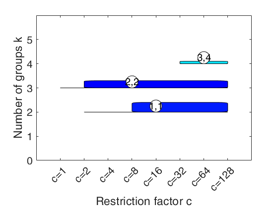
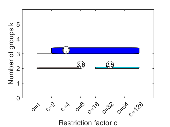
carbikeplot takes as input the output of function tclustICsol (that is a structure containing the best relevant solutions) and produces the car-bike plot. This plot provides a concise summary of the best relevant solutions. This plot shows on the horizontal axis the value of $c$ restriction factor (or $\alpha$ trimming level) and on the vertical axis the value of $k$. For each solution we draw a rectangle for the interval of values for which the solution is best and stable and a horizontal line which departs from the rectangle for the values of $c$ in which the solution is only stable. Finally, for the best value of $c$ ($\alpha$)associated to the solution, we show a circle with two numbers, the first number indicates the ranked solution among those which are not spurious and the second one the ranked number including the spurious solutions. This plot has been baptized ``car-bike'', because the first best solutions (in general 2 or 3) are generally best and stable for a large number of values of $c$ and therefore will have large rectangles. In addition, these solutions are likely to be stable for additional values of $c$ ($\alpha$) and therefore are likely to have horizontal lines departing from the rectangles (from here the name ``cars''). Finally, local minor solutions (which are associated with particular values of $c$ ($\alpha$) and $k$) do not generally present rectangles or lines and are shown with circles (from here the name ``bikes'')

example

h =carbikeplot(RelSol) Car-bike plot for simulated data.

example

h =carbikeplot(RelSol, Name, Value) car-bike plot for the geyser data.

example

[h, varargout] =carbikeplot(___) car-bike plot for the flea data.

Examples

expand all

  • Car-bike plot for simulated data.
  • Generate the data

    restrfact=5;
    rng('default') % Reinitialize the random number generator to its startup configuration
    rng(20000);
    ktrue=3;
    % n = number of observations
    n=150;
    % v= number of dimensions
    v=2;
    % Imposed average overlap
    BarOmega=0.04;
    out=MixSim(ktrue,v,'BarOmega',BarOmega, 'restrfactor',restrfact);
    % data generation given centroids and cov matrices
    [Y,id]=simdataset(n, out.Pi, out.Mu, out.S);
    nsamp=100;
    % Computation of information criterion
    out=tclustIC(Y,'cleanpool',false,'plots',0,'nsamp',nsamp);
    % Computation of the best solutions
    % Plot first 5 best solutions using as Information criterion CLACLA
    disp('Best 5 solutions using CLACLA')
    ThreshRandIndex=0.8;
    NumberOfBestSolutions=5;
    [outCLACLA]=tclustICsol(out,'whichIC','CLACLA','plots',0,'NumberOfBestSolutions',NumberOfBestSolutions,'ThreshRandIndex',ThreshRandIndex);
    % Car-bike plot to show what are the most relevant solutions
    carbikeplot(outCLACLA)
    Starting parallel pool (parpool) using the 'Processes' profile ...
    Connected to parallel pool with 8 workers.
    k=1
    k=2
    k=3
    k=4
    k=5
    Best 5 solutions using CLACLA
    
    ans = 
    
      Figure (1) with properties:
    
          Number: 1
            Name: ''
           Color: [0.9400 0.9400 0.9400]
        Position: [488 242 560 420]
           Units: 'pixels'
    
      Use GET to show all properties
    
    
    Click here for the graphical output of this example (link to Ro.S.A. website).

  • car-bike plot for the geyser data.
  • Y=load('geyser2.txt');
    nsamp=100;
    out=tclustIC(Y,'cleanpool',false,'plots',0,'alpha',0.1,'nsamp',nsamp);
    % Find the best solutions using as Information criterion MIXMIX
    disp('Best solutions using MIXMIX')
    [outMIXMIX]=tclustICsol(out,'whichIC','MIXMIX','plots',0,'NumberOfBestSolutions',6);
    % Produce the car-bike plot
    [h , sol_areas] = carbikeplot(outMIXMIX)
    k=1
    k=2
    k=3
    k=4
    k=5
    Best solutions using MIXMIX
    
    h = 
    
      Figure (2) with properties:
    
          Number: 2
            Name: ''
           Color: [0.9400 0.9400 0.9400]
        Position: [488 242 560 420]
           Units: 'pixels'
    
      Use GET to show all properties
    
    
    sol_areas =
    
        3.0000    0.0521
        4.0000         0
        5.0000         0
        5.0000         0
        2.0000    0.0052
        2.0000    0.0062
    
    
    Click here for the graphical output of this example (link to Ro.S.A. website).

  • car-bike plot for the flea data.
  • XX=load('flea.txt');
    Y=XX(:,1:end-1);
    nsamp=100;
    out=tclustIC(Y,'cleanpool',false,'plots',0,'alpha',0.1,'nsamp',nsamp);
    % Find the best solutions using as Information criterion CLACLA
    disp('Best solutions using CLACLA')
    [outCLACLA]=tclustICsol(out,'whichIC','CLACLA','plots',0,'NumberOfBestSolutions',6);
    % Produce the car-bike plot
    carbikeplot(outCLACLA);

    Input Arguments

    expand all

    RelSol — Relevant solutions produced by function tclustICsol. Structure.

    It contains the following fields:

    Value Description
    MIXMIXbs

    cell of size NumberOfBestSolutions-times-5 which contains the details of the best solutions for MIXMIX (BIC).

    Each row refers to a solution. The information which is stored in the columns is as follows.

    1st col = scalar, value of $k$ for which solution takes place;

    2nd col = scalar, value of $c$ ($\alpha$) for which solution takes place;

    3rd col = row vector of length d which contains the values of c for which the solution is uniformly better.

    4th col = row vector of length d+r which contains the values of c for which the solution is considered stable (i.e. for which the value of the adjusted Rand index (or the adjusted Fowlkes and Mallows index) does not go below the threshold defined in input option ThreshRandIndex).

    5th col = string which contains 'true' or 'spurious'. The solution is labelled spurious if the value of the adjusted Rand index with the previous solutions is greater than ThreshRandIndex.

    Remark: field out.MIXMIXbs is present only if input option 'whichIC' is 'ALL' or 'whichIC' is 'MIXMIX'.

    MIXMIXbsari

    matrix of adjusted Rand indexes (or Fowlkes and Mallows indexes) associated with the best solutions for MIXMIX. Matrix of size NumberOfBestSolutions-times-NumberOfBestSolutions whose i,j-th entry contains the adjusted Rand index between classification produced by solution i and solution j, $i,j=1, 2, \ldots, NumberOfBestSolutions$.

    Remark: field out.MIXMIXbsari is present only if 'whichIC' is 'ALL' or 'whichIC' is 'MIXMIX'.

    MIXCLAbs

    this output has the same structure as out.MIXMIXbs but it is referred to MIXCLA.

    Remark: field out.MIXCLAbs is present only if 'whichIC' is 'ALL' or 'whichIC' is 'MIXCLA'.

    MIXCLAbsari

    this output has the same structure as out.MIXMIXbs but it is referred to MIXCLA.

    Remark: field out.MIXCLAbsari is present only if 'whichIC' is 'ALL' or 'whichIC' is 'MIXCLA'.

    CLACLAbs

    this output has the same structure as out.MIXMIXbs but it is referred to CLACLA.

    Remark: field out.CLACLAbs is present only if 'whichIC' is 'ALL' or 'whichIC' is 'CLACLA'.

    CLACLAbsari

    this output has the same structure as out.MIXMIXbs but it is referred to CLACLA.

    Remark: field out.MIXCLAbsari is present only if 'whichIC' is 'ALL' or 'whichIC' is 'CLACLA'

    kk

    vector containing the values of k (number of components) which have been considered.

    cc

    scalar or vector containing the values of c (values of the restriction factor) which have been considered.

    Data Types: struct

    Name-Value Pair Arguments

    Specify optional comma-separated pairs of Name,Value arguments. Name is the argument name and Value is the corresponding value. Name must appear inside single quotes (' '). You can specify several name and value pair arguments in any order as Name1,Value1,...,NameN,ValueN.

    Example: 'SpuriousSolutions',false , 'minCarHeight',0.3

    SpuriousSolutions —Include or nor spurious solutions.boolean.

    As default spurios solutions are not included into the plot.

    Example: 'SpuriousSolutions',false

    Data Types: logical

    minCarHeight —minimum height of the rectangles in the carbike plot.positive numeric value.

    It can take values in the interval (0 1). Default value 0.1.

    Example: 'minCarHeight',0.3

    Data Types: single | double

    Output Arguments

    expand all

    h —graphics handle to the plot. Graphics handle

    Graphics handle which is produced on the screen.

    varargout —area : RelSol x 2 array reporting information on the relevance of the RelSol solutions. Each row corresponds to a solution for a given $k$

    The value of $k$ is in the first column. The area of the "car" rectangle of that $k$ solution is in the second column. The bigger the area, the better the solution (in terms of relevance and stability). This is a rule of thumb that can be used to select the optimal solutions in a semi-automatic way.

    References

    Cerioli, A. Garcia-Escudero, L.A., Mayo-Iscar, A. and Riani, M. (2017), Finding the Number of Groups in Model-Based Clustering via Constrained Likelihoods, "Journal of Computational and Graphical Statistics", pp. 404-416, https://doi.org/10.1080/10618600.2017.1390469

    This page has been automatically generated by our routine publishFS