
|
cabc |
carbikeplotGPCM |
 |
carbikeplot
carbikeplot produces the carbike plot to find best relevant clustering solutions
Syntax
Description
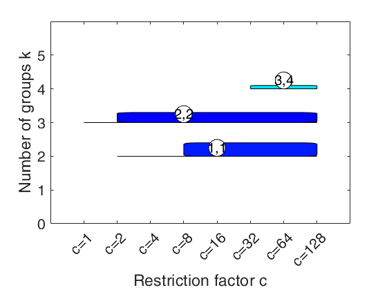
carbikeplot takes as input the output of function tclustICsol (that is a structure containing the best relevant solutions) and produces the car-bike plot. This plot provides a concise summary of the best relevant solutions. This plot shows on the horizontal axis the value of restriction factor (or \alpha trimming level) and on the vertical axis the value of k. For each solution we draw a rectangle for the interval of values for which the solution is best and stable and a horizontal line which departs from the rectangle for the values of c in which the solution is only stable. Finally, for the best value of c (\alpha)associated to the solution, we show a circle with two numbers, the first number indicates the ranked solution among those which are not spurious and the second one the ranked number including the spurious solutions. This plot has been baptized ``car-bike'', because the first best solutions (in general 2 or 3) are generally best and stable for a large number of values of c and therefore will have large rectangles. In addition, these solutions are likely to be stable for additional values of c (\alpha) and therefore are likely to have horizontal lines departing from the rectangles (from here the name ``cars''). Finally, local minor solutions (which are associated with particular values of c (\alpha) and k) do not generally present rectangles or lines and are shown with circles (from here the name ``bikes'')
car-bike plot for the geyser data.h
=carbikeplot(RelSol,
Name, Value)
Examples
 Car-bike plot for simulated data.
Car-bike plot for simulated data.Generate the data
restrfact=5;
rng('default') % Reinitialize the random number generator to its startup configuration
rng(20000);
ktrue=3;
% n = number of observations
n=150;
% v= number of dimensions
v=2;
% Imposed average overlap
BarOmega=0.04;
out=MixSim(ktrue,v,'BarOmega',BarOmega, 'restrfactor',restrfact);
% data generation given centroids and cov matrices
[Y,id]=simdataset(n, out.Pi, out.Mu, out.S);
nsamp=100;
% Computation of information criterion
out=tclustIC(Y,'cleanpool',false,'plots',0,'nsamp',nsamp);
% Computation of the best solutions
% Plot first 5 best solutions using as Information criterion CLACLA
disp('Best 5 solutions using CLACLA')
ThreshRandIndex=0.8;
NumberOfBestSolutions=5;
[outCLACLA]=tclustICsol(out,'whichIC','CLACLA','plots',0,'NumberOfBestSolutions',NumberOfBestSolutions,'ThreshRandIndex',ThreshRandIndex);
% Car-bike plot to show what are the most relevant solutions
carbikeplot(outCLACLA)
k=1
k=2
k=3
k=4
k=5
Best 5 solutions using CLACLA

ans =

  Figure (1) with properties:

      Number: 1
        Name: ''
       Color: [0.9400 0.9400 0.9400]
    Position: [488 242 560 420]
       Units: 'pixels'

  Use GET to show all properties
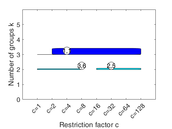
car-bike plot for the geyser data.
car-bike plot for the geyser data.
Y=load('geyser2.txt');
nsamp=100;
out=tclustIC(Y,'cleanpool',false,'plots',0,'alpha',0.1,'nsamp',nsamp);
% Find the best solutions using as Information criterion MIXMIX
disp('Best solutions using MIXMIX')
[outMIXMIX]=tclustICsol(out,'whichIC','MIXMIX','plots',0,'NumberOfBestSolutions',6);
% Produce the car-bike plot
[h , sol_areas] = carbikeplot(outMIXMIX)
k=1
k=2
k=3
k=4
k=5
Best solutions using MIXMIX

h =

  Figure (2) with properties:

      Number: 2
        Name: ''
       Color: [0.9400 0.9400 0.9400]
    Position: [488 242 560 420]
       Units: 'pixels'

  Use GET to show all properties


sol_areas =

    3.0000    0.0521
    4.0000         0
    5.0000         0
    5.0000         0
    2.0000    0.0052
    2.0000    0.0062
Input Arguments
Output Arguments
References
Cerioli, A. Garcia-Escudero, L.A., Mayo-Iscar, A. and Riani, M. (2017), Finding the Number of Groups in Model-Based Clustering via Constrained Likelihoods, "Journal of Computational and Graphical Statistics", pp. 404-416, https://doi.org/10.1080/10618600.2017.1390469
See Also
carbikeplotGPCM
|
tclustIC
|
tclustregIC
|
tclust
|
tclustICsol
|
tclustreg