tclustreg

tclustreg performs robust linear grouping analysis

expand all in page

Syntax

out=tclustreg(y,X,k,restrfact,alphaLik,alphaX)example
out=tclustreg(y,X,k,restrfact,alphaLik,alphaX,Name,Value)example
[out, varargout]=tclustreg(___)example

Description

example

out =tclustreg(y, X, k, restrfact, alphaLik, alphaX) tclustreg of 'X data'.

example

out =tclustreg(y, X, k, restrfact, alphaLik, alphaX, Name, Value) tclustreg of fishery data 1.

example

[out, varargout] =tclustreg(___) tclustreg of fishery data 2.

Examples

expand all

tclustreg of 'X data'.

The X data have been introduced by Gordaliza, Garcia-Escudero & Mayo-Iscar (2013).

% The dataset presents two parallel components without contamination.
X  = load('X.txt');
y1 = X(:,end);
X1 = X(:,1:end-1);
k = 2 ;
restrfact = 5; alpha1 = 0.05 ; alpha2 = 0.01;
out = tclustreg(y1,X1,k,restrfact,alpha1,alpha2);
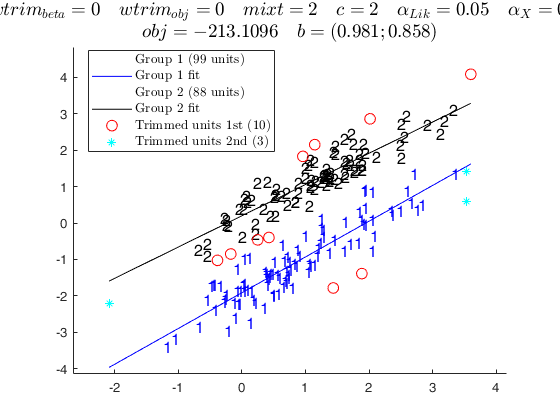
restrfact = 2; alpha1 = 0.05 ; alpha2 = 0.01;
out = tclustreg(y1,X1,k,restrfact,alpha1,alpha2,'mixt',2);
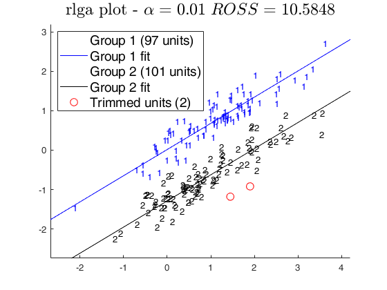
% Comparison with robust linear grouping
out = rlga(X,k,alpha2);
cascade;

ClaLik with untrimmed units selected using crisp criterion
Total estimated time to complete tclustreg:  1.15 seconds 
MixLik with untrimmed units selected using h largest lik contributions
Total estimated time to complete tclustreg:  0.85 seconds 
RLGA Algorithm k =2 biter =7 niter =10
Finished.

Click here for the graphical output of this example (link to Ro.S.A. website).

tclustreg of fishery data 1.

clear all; close all;
load fishery;
X = fishery{:,:};
% some jittering might be useful if there are many duplicated units
X = X + 10^(-8) * abs(randn(677,2));
%tclustreg on fishery data
y1 = X(:,end);
X1 = X(:,1:end-1);
k = 3 ; restrfact = 50; alpha1 = 0.04 ; alpha2 = 0.01;
out = tclustreg(y1,X1,k,restrfact,alpha1,alpha2,'intercept',0,'mixt',0);
title('TCLUST-REG');
%lga and rlga on fishery data
out=lga(X,3);
alpha = 0.95;
out=rlga(X,3,1-alpha);
cascade;

tclustreg of fishery data 2.

clear all; close all;
load fishery;
X = fishery{:,:};
% some jittering is necessary because duplicated units are not treated
% in tclustreg: this needs to be addressed
X = X + 10^(-8) * abs(randn(677,2));
y1 = X(:,end);
X1 = X(:,1:end-1);
% some arbitrary weights for the units
we = sqrt(X1)/sum(sqrt(X1));
% tclustreg required parameters
k = 2; restrfact = 50; alpha1 = 0.04 ; alpha2 = 0.01;
% now tclust is run on each combination of mixt and wtrim options
disp('mixt = 0; wtrim = 0;');
disp('standard tclustreg, with classification likelihood and without thinning' );
mixt = 0; wtrim = 0;
out = tclustreg(y1,X1,k,restrfact,alpha1,alpha2,'intercept',0,'mixt',mixt,'wtrim',wtrim);
disp('mixt = 2; wtrim = 0;');
disp('mixture likelihood, no thinning' );
mixt = 2; wtrim = 0;
out = tclustreg(y1,X1,k,restrfact,alpha1,alpha2,'intercept',0,'mixt',mixt,'wtrim',wtrim);
disp('mixt = 0; wtrim = 1;');
disp('classification likelihood, thinning based on user weights' );
mixt = 0; wtrim = 1;
out = tclustreg(y1,X1,k,restrfact,alpha1,alpha2,'intercept',0,'mixt',mixt,'we',we,'wtrim',wtrim);
disp('mixt = 2; wtrim = 1;');
disp('mixture likelihood, thinning based on user weights' );
mixt = 2; wtrim = 1;
out = tclustreg(y1,X1,k,restrfact,alpha1,alpha2,'intercept',0,'mixt',mixt,'we',we,'wtrim',wtrim);
disp('mixt = 0; wtrim = 2;');
disp('classification likelihood, thinning based on retention probabilities' );
mixt = 0; wtrim = 2; we = [];
out = tclustreg(y1,X1,k,restrfact,alpha1,alpha2,'intercept',0,'mixt',mixt,'wtrim',wtrim);
disp('mixt = 2; wtrim = 2;');
disp('mixture likelihood, thinning based on retention probabilities' );
mixt = 2; wtrim = 2; we = [];
out = tclustreg(y1,X1,k,restrfact,alpha1,alpha2,'intercept',0,'mixt',mixt,'wtrim',wtrim);
disp('mixt = 0; wtrim = 3;');
disp('classification likelihood, thinning based on bernoulli weights' );
mixt = 0; wtrim = 3; we = [];
out = tclustreg(y1,X1,k,restrfact,alpha1,alpha2,'intercept',0,'mixt',mixt,'wtrim',wtrim);
disp('mixt = 2; wtrim = 3;');
disp('mixture likelihood, thinning based on bernoulli weights' );
mixt = 2; wtrim = 3; we = [];
out = tclustreg(y1,X1,k,restrfact,alpha1,alpha2,'intercept',0,'mixt',mixt,'wtrim',wtrim);
disp('mixt = 0; wtrim = 4;');
disp('classification likelihood, tandem thinning based on bernoulli weights' );
mixt = 0; wtrim = 4; we = [];
out = tclustreg(y1,X1,k,restrfact,alpha1,alpha2,'intercept',0,'mixt',mixt,'wtrim',wtrim);
disp('mixt = 2; wtrim = 4;');
disp('mixture likelihood, tandem thinning based on bernoulli weights' );
mixt = 2; wtrim = 4; we = [];
out = tclustreg(y1,X1,k,restrfact,alpha1,alpha2,'intercept',0,'mixt',mixt,'wtrim',wtrim);
disp('mixt = 0; wtrim = struct; wtrim.wtype_beta=3;  wtrim.wtype_obj=''Z'';')
disp('classification likelihood, componentwise thinning based on bernoulli weights, objective function based on bernoulli weights' );
mixt = 0; wtrim = struct; wtrim.wtype_beta=3;  wtrim.wtype_obj='Z';
out = tclustreg(y1,X1,k,restrfact,alpha1,alpha2,'intercept',0,'mixt',mixt,'wtrim',wtrim);
disp('mixt = 0; wtrim = struct; wtrim.wtype_beta=2;  wtrim.wtype_obj=''w'';')
disp('classification likelihood, componentwise thinning based on retention probabilities, objective function based on retention probabilities' );
mixt = 0; wtrim = struct; wtrim.wtype_beta=2;  wtrim.wtype_obj='w';
out = tclustreg(y1,X1,k,restrfact,alpha1,alpha2,'intercept',0,'mixt',mixt,'wtrim',wtrim);
cascade

Related Examples

expand all

tclustreg of simulated data 1.

Generate mixture of regression using MixSimReg, with an average overlapping at centroids = 0.01. Use all default options.

rng(372,'twister');
p=3;
k=2;
Q=MixSimreg(k,p,'BarOmega',0.001);
n=500;
[y,X,id]=simdatasetreg(n,Q.Pi,Q.Beta,Q.S,Q.Xdistrib);
% plot the dataset
yXplot(y,X);
% run tclustreg
out=tclustreg(y,X(:,2:end),k,50,0.01,0.01,'intercept',1);

tclustreg of simulated data 2.

Generate mixture of regression using MixSimReg, with an average overlapping at centroids =0.01.

rng(372,'twister');
p=3;
k=2;
Q=MixSimreg(k,p,'BarOmega',0.001);
n=200;
[y,X,id]=simdatasetreg(n,Q.Pi,Q.Beta,Q.S,Q.Xdistrib);
% plot the dataset
yXplot(y,X);
% Generate the elemental subsets used in tclustreg once and for all.
nsamp  = 100;
ncomb  = bc(n,p);
method = [10*ones(n/2,1); ones(n/2,1)]; % weighted sampling using weights in "method"
msg    = 0;
for i=1:k
C(:,(i-1)*p+1:i*p) = subsets(nsamp, n, p, ncomb, msg, method);
end
% tclustreg using samples in C
out=tclustreg(y,X(:,2:end),k,50,0.01,0.01,'nsamp',C);

Example of nsamp passed as a matrix.

X  = load('X.txt');
y1 = X(:,end);
X1 = X(:,1:end-1);
n = 200;
k = 2 ;
restrfact = 5; alpha1 = 0.05 ; alpha2 = 0.01;
nsamp=200;
Cnsamp=subsets(nsamp,n,(size(X1,2)+1)*k);
out = tclustreg(y1,X1,k,restrfact,alpha1,alpha2,'nsamp',Cnsamp);

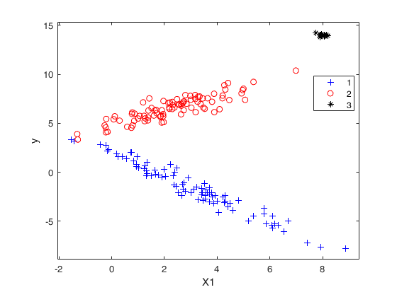
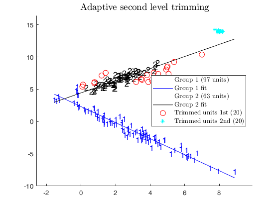
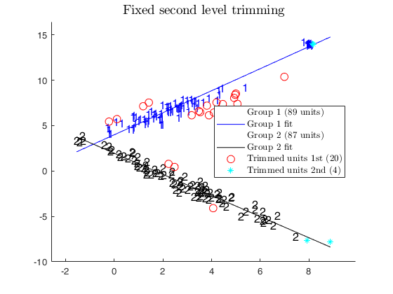
CWM, adaptive and fixed 2nd level trimming.

Comparison among CWM, adaptive second level trimming and fixed second level trimming

close all
% Generate two groups and a set of concentrated outliers
rng('default')
rng(100)
p=1;
n1=90;
x1=(randn(n1,p)+2)*2.1-1;
y1=-1.2*x1*1+randn(n1,1)*0.6+2.1;
n2=90;
x2=(randn(n1,p)+4)*1.5-4;
y2=5+x2*0.7+randn(n2,p)*0.6;
n3=20;
x3=randn(n3,p)*0.1+12-4;
y3=randn(n3,p)*0.1+16-2;
%x3=0;
%y3=0;
X=[x1;x2;x3];
y=[y1;y2;y3];
n=n1+n2+n3;
group=[ones(n1,1); 2*ones(n2,1); 3*ones(n3,1)];
yXplot(y,X,group);
legend('Location','best')
% gscatter(X,y,group)
% Run the 3 models and compare the results
k=2;
% Specify restriction factor for variance of residuals
restrfact=5;
% 10 per cent first level trimming.
alphaLik=0.1;
% number of subsamples to extract
nsamp=1000;
addnoisevariable = false;
if addnoisevariable ==true
X=[X randn(n,1)];
end
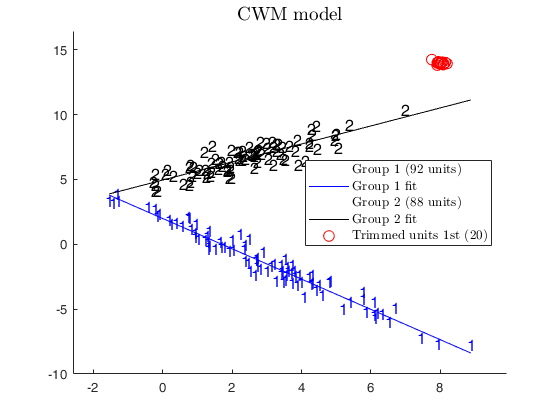
% In this case we use CWM model
alphaXcwm=1;
[outCWM]=tclustreg(y,X,k,restrfact,alphaLik,alphaXcwm,...
'mixt',0,'plots',1,'msg',0,'nsamp',nsamp);
title('CWM model')
% In this case we use an adaptive second level of trimming.
alphaXada=0.95;
[outADA]=tclustreg(y,X,k,restrfact,alphaLik,alphaXada,...
'mixt',0,'plots',1,'msg',0,'nsamp',nsamp);
title('Adaptive second level trimming')
% In this case we use a fixed level of trimming
alphaXfixed=0.02;
% Return in matrix X subsets used.
[out,C]=tclustreg(y,X,k,restrfact,alphaLik,alphaXfixed,...
'mixt',0,'plots',1,'msg',0,'nsamp',nsamp);
title('Fixed second level trimming')
disp('CWM model and adaptive second level trimming')
disp('can recover the real structure of the data')

CWM model and adaptive second level trimming
can recover the real structure of the data

tclustreg of fishery with commonslope.

clear all; close all;
load fishery;
X = fishery{:,:};
% some jittering might be useful if there are many duplicated units
X = X + 10^(-8) * abs(randn(677,2));
% Take the log of both variables
y1 = log(X(:,end));
X1 = log(X(:,1:end-1));
% tclustreg without commonslope and right number of groups
rng(12345);
% common parameters: number of groups overestimated
k = 5 ; restrfact = 50; alpha1 = 0.04 ; alpha2 = 0.01;
outlog = tclustreg(y1,X1,3,restrfact,alpha1,alpha2,'intercept',1,'commonslope',false,'mixt',0);
title({'TCLUST-REG on log without commonslope and k=3 (right number)',...
['estimated prices: ' num2str(exp(outlog.bopt(1,:)))] , ...
['estimated slopes: ' num2str(outlog.bopt(2,:))] });
xlim([-5 5]);
% tclustreg without commonslope
rng(12345);
outlogcsn = tclustreg(y1,X1,k,restrfact,alpha1,alpha2,'intercept',1,'commonslope',false,'mixt',0);
title({'TCLUST-REG on log without commonslope and k=5 (overestimated)',...
['estimated prices: ' num2str(exp(outlogcsn.bopt(1,:)))] , ...
['estimated slopes: ' num2str(outlogcsn.bopt(2,:))] });
xlim([-5 5]);
% tclustreg with commonslope 
rng(12345);
outlogcsy = tclustreg(y1,X1,k,restrfact,alpha1,alpha2,'intercept',1,'commonslope',true,'mixt',0);
title({'TCLUST-REG on log with commonslope and k=5 (overestimated)',...
['estimated prices: ' num2str(exp(outlogcsy.bopt(1,:)))] , ...
['estimated slopes: ' num2str(outlogcsy.bopt(2,:))] });
xlim([-5 5]);
cascade;

Input Arguments

expand all

`y` — Response variable. Vector.

A vector with n elements that contains the response variable.

y can be either a row or a column vector.

Data Types: single|double

`X` — Explanatory variables (also called 'regressors'). Matrix.

Data matrix of dimension $(n \times p-1)$. Rows of X represent observations, and columns represent variables. Missing values (NaN's) and infinite values (Inf's) are allowed, since observations (rows) with missing or infinite values will automatically be excluded from the computations.

Data Types: single|double

`k` — Number of clusters. Scalar.

This is a guess on the number of data groups.

Data Types: single|double

`restrfact` — restriction factor for regression residuals and covariance matrices of the explanatory variables. Scalar or vector with two elements.

If restrfact is a scalar it controls the differences among group scatters of the residuals. The value 1 is the strongest restriction. If restrfactor is a vector with two elements the first element controls the differences among group scatters of the residuals and the second the differences among covariance matrices of the explanatory variables. Note that restrfactor(2) is used just if input option $alphaX=1$, that is if constrained weighted model for X is assumed.

Data Types: single|double

`alphaLik` — Trimming level. Scalar.

alphaLik is a value between 0 and 0.5 or an integer specifying the number of observations which have to be trimmed. If alphaLik=0 there is no trimming. More in detail, if 0<alphaLik<1 clustering is based on h=fix(n*(1-alphaLik)) observations.

Else if alphaLik is an integer greater than 1 clustering is based on h=n-floor(alphaLik). More in detail, likelihood contributions are sorted and the units associated with the smallest n-h contributions are trimmed.

Data Types: single|double

`alphaX` — Second-level trimming or constrained weighted model for X. Scalar.

alphaX is a value in the interval [0 1].

- If alphaX=0 there is no second-level trimming.

- If alphaX is in the interval [0 0.5] it indicates the fixed proportion of units subject to second level trimming.

In this case alphaX is usually smaller than alphaLik.

For further details see Garcia-Escudero et. al. (2010).

- If alphaX is in the interval (0.5 1), it indicates a Bonferronized confidence level to be used to identify the units subject to second level trimming. In this case the proportion of units subject to second level trimming is not fixed a priori, but is determined adaptively.

For further details see Torti et al. (2018).

- If alphaX=1, constrained weighted model for X is assumed (Gershenfeld, 1997). The CWM estimator is able to take into account different distributions for the explanatory variables across groups, so overcoming an intrinsic limitation of mixtures of regression, because they are implicitly assumed equally distributed. Note that if alphaX=1 it is also possible to apply using restrfactor(2) the constraints on the cov matrices of the explanatory variables.

For further details about CWM see Garcia-Escudero et al.

(2017) or Torti et al. (2018).

Data Types: single|double

Name-Value Pair Arguments

Specify optional comma-separated pairs of Name,Value arguments. Name is the argument name and Value is the corresponding value. Name must appear inside single quotes (' '). You can specify several name and value pair arguments in any order as Name1,Value1,...,NameN,ValueN.

Example:

 'intercept',1
, 'mixt',1
, 'equalweights',true
, 'nsamp',1000
, 'refsteps',15
, 'reftol',1e-05
, 'commonslope',true
, 'plots',1
, 'wtrim',1
, 'we',[0.2 0.2 0.2 0.2 0.2]
, cup, 0.8
, pstar, 0.95
, 'k_dens_mixt',6
, 'nsamp_dens_mixt',1000
, 'refsteps_dens_mixt',15
, 'method_dens_mixt','E'
, 'msg',1
, 'RandNumbForNini',''
, 'nocheck',1

`intercept` —Indicator for constant term.scalar.

If 1, a model with constant term will be fitted (default), else no constant term will be included.

Example: 'intercept',1

Data Types: double

`mixt` —mixture modelling or crisp assignment.scalar.

Option mixt specifies whether mixture modelling or crisp assignment approach to model based clustering must be used.

In the case of mixture modelling parameter mixt also controls which is the criterior to find the untrimmed units in each step of the maximization If mixt >=1 mixture modelling is assumed else crisp assignment.

In mixture modelling the likelihood is given by

\[ \prod_{i=1}^n \sum_{j=1}^k \pi_j \phi (y_i \; x_i' , \beta_j , \sigma_j), \] while in crisp assignment the likelihood is given by \[ \prod_{j=1}^k \prod _{i\in R_j} \pi_j \phi (y_i \; x_i' , \beta_j , \sigma_j), \]

where $R_j$ contains the indexes of the observations which are assigned to group $j$, Remark - if mixt>=1 previous parameter equalweights is automatically set to 1.

Parameter mixt also controls the criterion to select the units to trim if mixt == 2 the h units are those which give the largest contribution to the likelihood that is the h largest values of

\[ \sum_{j=1}^k \pi_j \phi (y_i \; x_i' , \beta_j , \sigma_j) \qquad i=1, 2, ..., n \] elseif mixt==1 the criterion to select the h units is exactly the same as the one which is used in crisp assignment. That is: the n units are allocated to a cluster according to criterion \[ \max_{j=1, \ldots, k} \hat \pi'_j \phi (y_i \; x_i' , \beta_j , \sigma_j) \]

and then these n numbers are ordered and the units associated with the largest h numbers are untrimmed.

Example: 'mixt',1

Data Types: single | double

`equalweights` —cluster weights in the concentration and assignment steps.logical.

A logical value specifying whether cluster weights shall be considered in the concentration, assignment steps and computation of the likelihood.

if equalweights = true we are (ideally) assuming equally sized groups by maximizing the likelihood. Default value false.

Example: 'equalweights',true

Data Types: Logical

`nsamp` —number of subsamples to extract.scalar | matrix with k*p columns.

If nsamp is a scalar it contains the number of subsamples which will be extracted.

If nsamp=0 all subsets will be extracted.

If the number of all possible subset is <300 the default is to extract all subsets, otherwise just 300.

If nsamp is a matrix it contains in the rows the indexes of the subsets which have to be extracted. nsamp in this case can be conveniently generated by function subsets.

nsamp must have k*p columns. The first p columns are used to estimate the regression coefficient of group 1... the last p columns are used to estimate the regression coefficient of group k

Example: 'nsamp',1000

Data Types: double

`refsteps` —Number of refining iterations.scalar.

Number of refining iterations in each subsample. Default is 10.

refsteps = 0 means "raw-subsampling" without iterations.

Example: 'refsteps',15

Data Types: single | double

`reftol` —Tolerance for the refining steps.scalar.

The default value is 1e-14;

Example: 'reftol',1e-05

Data Types: single | double

`commonslope` —Impose constraint of common slope regression coefficients.boolean.

If commonslope is true, the groups are forced to have the same regression coefficients (apart from the intercepts).

The default value of commonslope is false;

Example: 'commonslope',true

Data Types: boolean

`plots` —Plot on the screen.scalar.

A flag to control the generation of the plots.

If plots=1 a plot is showed on the screen with the final allocation (and if size(X,2)==2 with the lines associated to the groups)

Example: 'plots',1

Data Types: double

`wtrim` —Application of observation weights.scalar | structure.

If wtrim is a scalar, a flag taking values in [0, 1, 2, 3, 4], to control the application of weights on the observations for betaestimation.

- If \texttt{wtrim}=0 (no weights) and $\texttt{mixt}=0$, the algorithm reduces to the standard tclustreg algorithm.

- If \texttt{wtrim}=0 and \texttt{mixt}=2, the maximum posterior probability $D_i$ of equation 7 of Garcia et al. 2010 is computing by maximizing the log-likelihood contributions of the mixture model of each observation.

- If \texttt{wtrim} = 1, trimming is done by weighting the observations using values specified in vector \texttt{we}.

In this case, vector \texttt{we} must be supplied by the user. For instance, \texttt{we} = $X$.

- If \texttt{wtrim} = 2, trimming is again done by weighting the observations using values specified in vector \texttt{we}.

In this case, vector \texttt{we} is computed from the data as a function of the density estimate $\mbox{pdfe}$.

Specifically, the weight of each observation is the probability of retaining the observation, computed as

\[\mbox{pretain}_{i g} = 1 - \mbox{pdfe}_{ig}/\max_{ig}(\mbox{pdfe}_{ig})\]

- If \texttt{wtrim} = 3, trimming is again done by weighting the observations using values specified in vector \texttt{we}. In this case, each element $we_i$ of vector \texttt{we} is a Bernoulli random variable with probability of success $\mbox{pdfe}_{ig}$. In the clustering framework this is done under the constraint that no group is empty.

- If \texttt{wtrim} = 4, trimming is done with the tandem approach of Cerioli and Perrotta (2014).

- If \texttt{wtrim} = 5 (TO BE IMPLEMENTED) - If \texttt{wtrim} = 6 (TO BE IMPLEMENTED) If wtrim is a structure, it is composed by: - wtrim.wtype_beta: the weight for the beta estimation. It can be 0, 1, 2, 3, as in the case of wtrim scalar - wtrim.wtype_obj: the weight for the objective function. It can be: - '0': no weights in the objective function - 'Z': Bernoulli random variable with probability of success $\mbox{pdfe}_{ig}$ - 'w': a function of the density estimate $\mbox{pdfe}$.

- 'Zw': the product of the two above.

- 'user': user weights we.

Example: 'wtrim',1

Data Types: double

`we` —Vector of observation weights.vector.

A vector of size n-by-1 containing application-specific weights that the user needs to apply to each observation. Default value is a vector of ones.

Example: 'we',[0.2 0.2 0.2 0.2 0.2]

Data Types: double

`cup` —pdf upper limit.scalar.

The upper limit for the pdf used to compute the retantion probability. If cup = 1 (default), no upper limit is set.

Example: cup, 0.8

Data Types: scalar

`pstar` —thinning probability.scalar.

Probability with each a unit enters in the thinning procedure. If pstar = 1 (default), all units enter in the thinning procedure.

Example: pstar, 0.95

Data Types: scalar

`k_dens_mixt` —in the Poisson/Exponential mixture density function, number of clusters for density mixtures.scalar.

This is a guess on the number of data groups. Default value is 5.

Example: 'k_dens_mixt',6

Data Types: single|double

`nsamp_dens_mixt` —in the Poisson/Exponential mixture density function, number of subsamples to extract.scalar.

Default 300.

Example: 'nsamp_dens_mixt',1000

Data Types: double

`refsteps_dens_mixt` —in the Poisson/Exponential mixture density function, number of refining iterations.scalar.

Number of refining iterations in each subsample. Default is 10.

Example: 'refsteps_dens_mixt',15

Data Types: single | double

`method_dens_mixt` —in the Poisson/Exponential mixture density function, distribution to use.character.

If method_dens_mixt = 'P', the Poisson distribution is used, with method_dens_mixt = 'E', the Exponential distribution is used. Default is 'P'.

Example: 'method_dens_mixt','E'

Data Types: char

`msg` —Level of output to display.scalar.

Scalar which controls whether to display or not messages on the screen.

If msg==0 nothing is displayed on the screen.

If msg==1 (default) messages are displayed on the screen about estimated time to compute the estimator or the number of subsets in which there was no convergence.

If msg==2 detailed messages are displayed. For example the information at iteration level.

Example: 'msg',1

Data Types: single | double

`RandNumbForNini` —Pre-extracted random numbers to initialize proportions.matrix.

Matrix with size k-by-size(nsamp,1) containing the random numbers which are used to initialize the proportions of the groups. This option is effective just if nsamp is a matrix which contains pre-extracted subsamples. The purpose of this option is to enable the user to replicate the results in case routine tclust is called using a parfor instruction (as it happens for example in routine IC, where tclust is called through a parfor for different values of the restriction factor).

The default value of RandNumbForNini is empty that is random numbers from uniform are used.

Example: 'RandNumbForNini',''

Data Types: single | double

`nocheck` —Check input arguments.scalar.

If nocheck is equal to 1 no check is performed on vector y and matrix X.

As default nocheck=0.

Example: 'nocheck',1

Data Types: single | double

Output Arguments

expand all

`out` — description Structure

Structure containing the following fields

Value	Description
`bopt`	$(p+1) \times k$ matrix containing the regression parameters.
`sigma2opt`	$k$ row vector containing the estimated group variances.
`sigma2opt_corr`	$k$ row vector containing the estimated group variances corrected with asymptotic consistency factor.
`muXopt`	k-by-p matrix containing cluster centroid locations. Robust estimate of final centroids of the groups. This output is present only if input option alphaX is 1.
`sigmaXopt`	p-by-p-by-k array containing estimated constrained covariance covariance matrices of the explanatory variables for the k groups. This output is present only if input option alphaX is 1.
`cstepopt`	scalar containing the concentration step where the objective function was the largest. This is useful when the objective function is not monotone (e.g. with second level trimming or with thinning).
`subsetopt`	scalar containing the subset id where the objective function was the largest.
`idx`	n-by-1 vector containing assignment of each unit to each of the k groups. Cluster names are integer numbers from -2 to k. -1 indicates first level trimmed units. -2 indicates second level trimmed units.
`siz`	Matrix of size k-by-3. 1st col = sequence from -2 to k; 2nd col = number of observations in each cluster; 3rd col = percentage of observations in each cluster; Remark: 0 denotes thinned units (if the weights to find thinned units are 0 or 1, -1 indicates first level trimmed units and -2 indicates second level trimmed units).
`postprobopt`	$n \times k$ matrix containing the final posterior probabilities. out.postprobopt(i,j) contains posterior probabilitiy of unit i from component (cluster) j. For the trimmed units posterior probabilities are 0. This output is always produced (independently of the value of mixt).
`MIXMIX`	BIC which uses parameters estimated using the mixture loglikelihood and the maximized mixture likelihood as goodness of fit measure. Remark: this output is present only if input option mixt is >0.
`MIXCLA`	BIC which uses the classification likelihood based on parameters estimated using the mixture likelihood (In some books this quantity is called ICL). This output is present only if input option mixt is >0.
`CLACLA`	BIC which uses the classification likelihood based on parameters estimated using the classification likelihood. Remark: this output is present only if input option mixt is =0.
`obj`	scalar containing value of the objective function.
`fullsol`	Column vector of size nsamp which contains the value of the objective function (maximized log likelihood) at the end of the iterative process for each extracted subsample. Note that max(out.fullsol) is equal to out.obj.
`NlogL`	Scalar. -2 log classification likelihood. In presence of full convergence -out.NlogL/2 is equal to out.obj.
`NlogLmixt`	Scalar. -2 log mixture likelihood. In presence of full convergence -out.NlogLmixt/2 is equal to out.obj. If input parameter mixt=0 then out.NlogLmixt is a missing value.
`h`	Scalar. Number of observations that have determined the regression coefficients (number of untrimmed units).
`class`	'tclustreg'.

`varargout` —C : Indexes of extracted subsamples. Matrix

Matrix of size nsamp-by-k*p containing (in the rows) the indices of the subsamples extracted for computing the estimate.

More About

expand all

Additional Details

Computational issues to be addressed in future releases.

[1] FSDA function "wthin" uses the MATLAB function ksdensity. The calls to ksdensity have been optimized. The only possibility to further reduce time execution is to replace ksdensity with a more efficient kernel density estimator.

[2] The weighted version of tclustreg requires weighted sampling. This is now implemented in randsampleFS. A computaionally more efficient algorithm, based on a binary tree approach introduced by Wong, C.K. and M.C. Easton (1980) "An Efficient Method for Weighted Sampling Without Replacement", SIAM Journal of Computing, 9(1):111-113.

is provided by recent releases of the MATLAB function datasample.

Unfortunately this function spends most of the self running time useless parameter checking. To copy the function in the FSDA folder FSDA/combinatorial, possibly rename it, and remove the option parameters checks, is not sufficient, as datasample relies on a mex file wswor which is platform dependent. The issue is usually referred to as "code signature".

[3] In the plots, the use of text to highlight the groups with their index is terribly slow (more than 10 seconds to generate a scatter of 7000 units. ClickableMultiLegend and legend are also slow.

[4] FSDA function restreigen could be improved. In some cases it is one of the most expensive functions.

REMARK: trimming vs thinning - trimming is the key feature of TCLUST, giving robustness to the model.

- thinning is a new denoising feature introduced to mitigate the distorting effect of very dense data areas. It is implemented via observation weighting.

For the sake of code readability, the relevant sections of the code are identified with a "TRIMMING" or "THINNING" tag.

REMARK: the number of parameters to penalize the likelihood are given below: $k(p+1)$ = number of regression coefficients including the intercept.

$k-1$ = number of proportions -1 (because their sum is 1).

$(k-1)(1-1/restrfact(1))+1$ = constraints on the $\sigma^2_j$.

To the above parameters, if $alphaX=1$ we must add: $k(p-1)p/2$ = rotation parameters for $\Sigma_X=cov(X)$.

$(kp-1)(1-1/restrfactor(2))+1$ = eigenvalue parameters for $\Sigma_X=cov(X)$.

References

Garcia-Escudero, L.A., Gordaliza A., Greselin F., Ingrassia S., and Mayo-Iscar A. (2016), The joint role of trimming and constraints in robust estimation for mixtures of gaussian factor analyzers, "Computational Statistics & Data Analysis", Vol. 99, pp. 131-147.

Garcia-Escudero, L.A., Gordaliza, A., Greselin, F., Ingrassia, S. and Mayo-Iscar, A. (2017), Robust estimation of mixtures of regressions with random covariates, via trimming and constraints, "Statistics and Computing", Vol. 27, pp. 377-402.

Garcia-Escudero, L.A., Gordaliza A., Mayo-Iscar A., and San Martin R. (2010), Robust clusterwise linear regression through trimming, "Computational Statistics and Data Analysis", Vol. 54, pp.3057-3069.

Cerioli, A. and Perrotta, D. (2014). Robust Clustering Around Regression Lines with High Density Regions. Advances in Data Analysis and Classification, Vol. 8, pp. 5-26.

Torti F., Perrotta D., Riani, M. and Cerioli A. (2019). Assessing Robust Methodologies for Clustering Linear Regression Data, "Advances in Data Analysis and Classification", Vol. 13, pp. 227–257, https://doi.org/10.1007/s11634-018-0331-4

tclustreg

Syntax

Description

Examples

Related Examples

Input Arguments

y — Response variable. Vector.

X — Explanatory variables (also called 'regressors'). Matrix.

k — Number of clusters. Scalar.

restrfact — restriction factor for regression residuals and covariance matrices of the explanatory variables. Scalar or vector with two elements.

alphaLik — Trimming level. Scalar.

alphaX — Second-level trimming or constrained weighted model for X. Scalar.

Name-Value Pair Arguments

intercept —Indicator for constant term.scalar.

mixt —mixture modelling or crisp assignment.scalar.

equalweights —cluster weights in the concentration and assignment steps.logical.

nsamp —number of subsamples to extract.scalar | matrix with k*p columns.

refsteps —Number of refining iterations.scalar.

reftol —Tolerance for the refining steps.scalar.

commonslope —Impose constraint of common slope regression coefficients.boolean.

plots —Plot on the screen.scalar.

wtrim —Application of observation weights.scalar | structure.

we —Vector of observation weights.vector.

cup —pdf upper limit.scalar.

pstar —thinning probability.scalar.

k_dens_mixt —in the Poisson/Exponential mixture density function, number of clusters for density mixtures.scalar.

nsamp_dens_mixt —in the Poisson/Exponential mixture density function, number of subsamples to extract.scalar.

refsteps_dens_mixt —in the Poisson/Exponential mixture density function, number of refining iterations.scalar.

method_dens_mixt —in the Poisson/Exponential mixture density function, distribution to use.character.

msg —Level of output to display.scalar.

RandNumbForNini —Pre-extracted random numbers to initialize proportions.matrix.

nocheck —Check input arguments.scalar.

Output Arguments

out — description Structure

varargout —C : Indexes of extracted subsamples. Matrix

More About

References

See Also

`y` — Response variable. Vector.

`X` — Explanatory variables (also called 'regressors'). Matrix.

`k` — Number of clusters. Scalar.

`restrfact` — restriction factor for regression residuals and covariance matrices of the explanatory variables. Scalar or vector with two elements.

`alphaLik` — Trimming level. Scalar.

`alphaX` — Second-level trimming or constrained weighted model for X. Scalar.

`intercept` —Indicator for constant term.scalar.

`mixt` —mixture modelling or crisp assignment.scalar.

`equalweights` —cluster weights in the concentration and assignment steps.logical.

`nsamp` —number of subsamples to extract.scalar | matrix with k*p columns.

`refsteps` —Number of refining iterations.scalar.

`reftol` —Tolerance for the refining steps.scalar.

`commonslope` —Impose constraint of common slope regression coefficients.boolean.

`plots` —Plot on the screen.scalar.

`wtrim` —Application of observation weights.scalar | structure.

`we` —Vector of observation weights.vector.

`cup` —pdf upper limit.scalar.

`pstar` —thinning probability.scalar.

`k_dens_mixt` —in the Poisson/Exponential mixture density function, number of clusters for density mixtures.scalar.

`nsamp_dens_mixt` —in the Poisson/Exponential mixture density function, number of subsamples to extract.scalar.

`refsteps_dens_mixt` —in the Poisson/Exponential mixture density function, number of refining iterations.scalar.

`method_dens_mixt` —in the Poisson/Exponential mixture density function, distribution to use.character.

`msg` —Level of output to display.scalar.

`RandNumbForNini` —Pre-extracted random numbers to initialize proportions.matrix.

`nocheck` —Check input arguments.scalar.

`out` — description Structure

`varargout` —C : Indexes of extracted subsamples. Matrix