tclust
tclust computes trimmed clustering with scatter restrictions
Syntax
Description
tclust partitions the points in the n-by-v data matrix Y into k clusters. This partition minimizes the trimmed sum, over all clusters, of the within-cluster sums of point-to-cluster-centroid distances. Rows of Y correspond to points, columns correspond to variables. tclust returns inside structure out an n-by-1 vector idx containing the cluster indices of each point. By default, tclust uses (squared), possibly constrained, Mahalanobis distances.
tclust of geyser data using k=3, alpha=0.1 and restrfactor=10000.out
=tclust(Y,
k,
alpha,
restrfactor)
Use of 'plots' option as a struct, to produce more complex plots.out
=tclust(Y,
k,
alpha,
restrfactor,
Name, Value)
Examples
tclust of geyser data using k=3, alpha=0.1 and restrfactor=10000.
Y=load('geyser2.txt');
out=tclust(Y,3,0.1,10000);
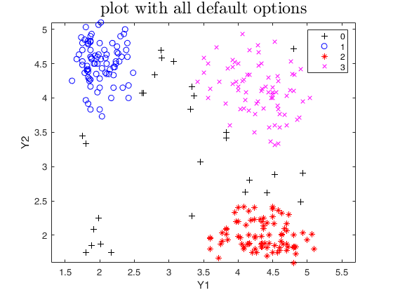
 Use of 'plots' option as a struct, to produce more complex plots.
Use of 'plots' option as a struct, to produce more complex plots.
Y=load('geyser2.txt');
close all
out=tclust(Y,3,0.1,10000,'plots',1);
title('plot with all default options','interpreter','LaTex','FontSize',18);
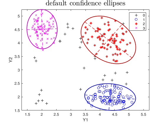
% default confidence ellipses.
out=tclust(Y,3,0.1,10000,'plots','ellipse');
title('default confidence ellipses','interpreter','LaTex','FontSize',18);
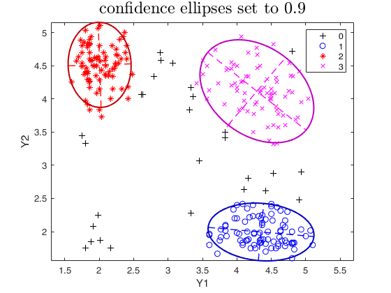
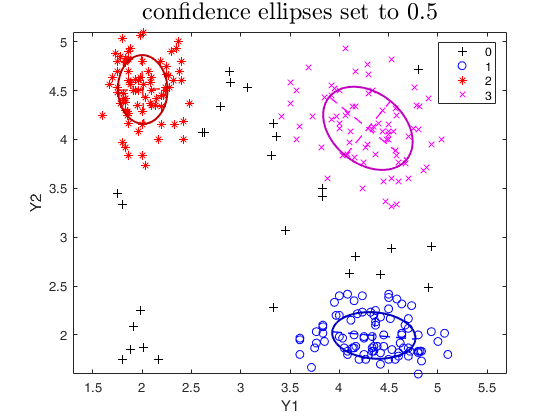
% confidence ellipses specified by the user
plots.type = 'ellipse';
plots.conflev = 0.5;
out=tclust(Y,3,0.1,10000,'plots',plots);
title('confidence ellipses set to 0.5','interpreter','LaTex','FontSize',18);
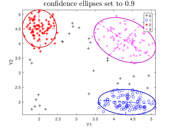
plots.conflev = 0.9;
out=tclust(Y,3,0.1,10000,'plots',plots);
title('confidence ellipses set to 0.9','interpreter','LaTex','FontSize',18);
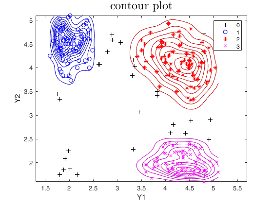
% contour plots.
out=tclust(Y,3,0.1,10000,'plots','contour');
title('contour plot','interpreter','LaTex','FontSize',18);
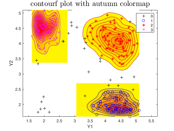
% filled contour plots with additional options
plots.type = 'contourf';
plots.cmap = autumn;
out=tclust(Y,3,0.1,10000,'plots',plots);
title('contourf plot with autumn colormap','interpreter','LaTex','FontSize',18);
cascade
ClaLik with untrimmed units selected using crisp criterion
Total estimated time to complete tclust:  0.66 seconds
ClaLik with untrimmed units selected using crisp criterion
Total estimated time to complete tclust:  0.21 seconds
ClaLik with untrimmed units selected using crisp criterion
Total estimated time to complete tclust:  0.19 seconds
ClaLik with untrimmed units selected using crisp criterion
Total estimated time to complete tclust:  0.18 seconds
ClaLik with untrimmed units selected using crisp criterion
Total estimated time to complete tclust:  0.15 seconds
ClaLik with untrimmed units selected using crisp criterion
Total estimated time to complete tclust:  0.23 seconds


tclust of geyser with varargout.
Y=load('geyser2.txt');
nsamp=20;
[out,MatrixContSubsets]=tclust(Y,3,0.1,10000,'nsamp',nsamp);
% MatrixContSubsets is a matrix containing in the rows the indexes of
% the nsamp subsets which have been extracted
Related Examples
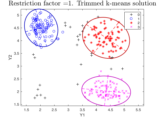
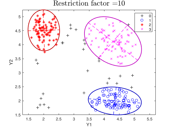
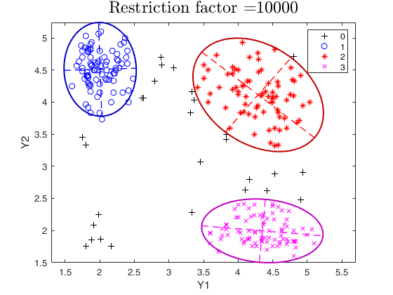
tclust of geyser data (output comparison).
tclust of geyser data (output comparison).We compare the output using three different values of restriction factor.
close all
Y=load('geyser2.txt');
restrfactor=10000;
% nsamp = number of subsamples which will be extracted
nsamp=500;
out=tclust(Y,3,0.1,restrfactor,'nsamp',nsamp,'plots','ellipse');
title(['Restriction factor =' num2str(restrfactor)],'interpreter','LaTex','FontSize',18)
restrfactor=10;
out=tclust(Y,3,0.1,restrfactor,'nsamp',nsamp,'refsteps',10,'plots','ellipse');
title(['Restriction factor =' num2str(restrfactor)],'interpreter','LaTex','FontSize',18)
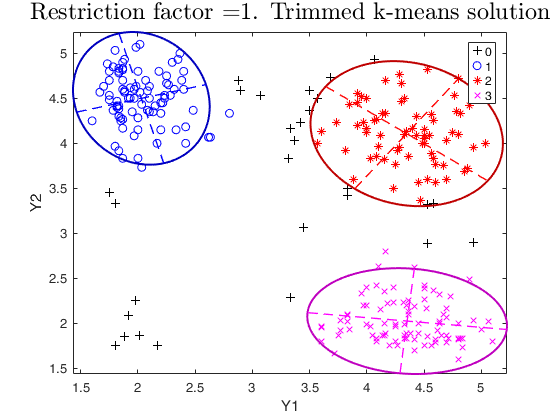
% trimmed k-means solution restrfactor=1
restrfactor=1;
out=tclust(Y,3,0.1,restrfactor,'nsamp',nsamp,'refsteps',10,'plots','ellipse');
title(['Restriction factor =' num2str(restrfactor) '. Trimmed k-means solution'],'interpreter','LaTex','FontSize',18)
cascade
ClaLik with untrimmed units selected using crisp criterion
Total estimated time to complete tclust:  0.26 seconds
ClaLik with untrimmed units selected using crisp criterion
Total estimated time to complete tclust:  0.35 seconds
ClaLik with untrimmed units selected using crisp criterion
Total estimated time to complete tclust:  0.32 seconds


tclust applied to the M5data.
A bivariate data set obtained from three normal bivariate distributions with different scales and proportions 1:2:2. One of the components is very overlapped with another one. A 10 per cent background noise is added uniformly distributed in a rectangle containing the three normal components and not very overlapped with the three mixture components. A precise description of the M5 data set can be found in Garcia-Escudero et al. (2008).
close all
Y=load('M5data.txt');
% plot(Y(:,1),Y(:,2),'o')
% Scatter plot matrix with univariate boxplot on the main diagonal
spmplot(Y(:,1:2),Y(:,3),[],'box');
out=tclust(Y(:,1:2),3,0,1000,'nsamp',100,'plots',1);
out=tclust(Y(:,1:2),3,0,10,'nsamp',100,'plots',1);
out=tclust(Y(:,1:2),3,0.1,1,'nsamp',1000,'plots',1,'equalweights',1);
out=tclust(Y(:,1:2),3,0.1,1000,'nsamp',100,'plots',1);
cascade
tclust in presence of structured noise.
The data have been generated using the following R instructions set.seed (0) library(MASS) v <- runif (100, -2 * pi, 2 * pi) noise <- cbind (100 + 25 * sin (v), 10 + 5 * v) x <- rbind ( rmvnorm (360, c (0.0, 0), matrix (c (1, 0, 0, 1), ncol = 2)), rmvnorm (540, c (5.0, 10), matrix (c (6, -2, -2, 6), ncol = 2)), noise)
close all
Y=load('structurednoise.txt');
out=tclust(Y(:,1:2),2,0.1,100,'plots',1);
out=tclust(Y(:,1:2),5,0.15,1,'plots',1);
cascade
tclust applied to mixture100 data.
The data have been generated using the following R instructions set.seed (100) mixt <- rbind (rmvnorm (360, c ( 0, 0), matrix (c (1, 0, 0, 1), ncol = 2)), rmvnorm (540, c ( 5, 10), matrix (c (6, -2, -2, 6), ncol = 2)), rmvnorm (100, c (2.5, 5), matrix (c (50, 0, 0, 50), ncol = 2)))
close all
Y=load('mixture100.txt');
out=tclust(Y(:,1:2),3,0.05,1000,'refsteps',20,'plots',1);
out=tclust(Y(:,1:2),3,0.05,1,'refsteps',20,'plots',1);
cascade
tclust applied to mixture100 data, comparison of different options.
close all
Y=load('mixture100.txt');
% Traditional tclust
out1=tclust(Y(:,1:2),3,0.05,1000,'refsteps',20,'plots',1);
title('Traditional tclust','interpreter','LaTex','FontSize',18);
% tclust with mixture models (selection of untrimmed units according to
% likelihood contributions
out2=tclust(Y(:,1:2),3,0.05,1000,'refsteps',20,'plots',1,'mixt',1);
title('tclust with mixture models (likelihood contributions)','interpreter','LaTex','FontSize',18);
% Tclust with mixture models (selection of untrimmed units according to
% densities weighted by estimates of the probability of the components)
out3=tclust(Y(:,1:2),3,0.05,1000,'refsteps',20,'plots',1,'mixt',2);
title('tclust with mixture models (probability of the components)','interpreter','LaTex','FontSize',18);
cascade
tclust using simulated data.
5 groups and 5 variables
n1=100;
n2=80;
n3=50;
n4=80;
n5=70;
v=5;
Y1=randn(n1,v)+5;
Y2=randn(n2,v)+3;
Y3=rand(n3,v)-2;
Y4=rand(n4,v)+2;
Y5=rand(n5,v);
group=ones(n1+n2+n3+n4+n5,1);
group(n1+1:n1+n2)=2;
group(n1+n2+1:n1+n2+n3)=3;
group(n1+n2+n3+1:n1+n2+n3+n4)=4;
group(n1+n2+n3+n4+1:n1+n2+n3+n4+n5)=5;
close all
Y=[Y1;Y2;Y3;Y4;Y5];
out=tclust(Y,5,0.05,1.3,'refsteps',20,'plots',1);
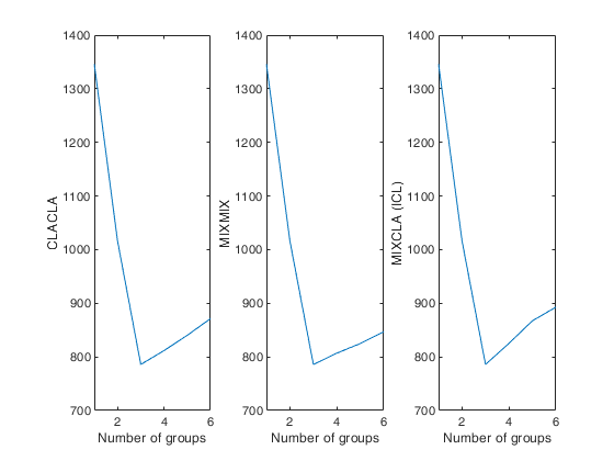
Automatic choice of the best number of groups for geyser data.
Automatic choice of the best number of groups for geyser data.close all
Y=load('geyser2.txt');
maxk=6;
CLACLA=[(1:maxk)' zeros(maxk,1)];
for j=1:maxk
out=tclust(Y,j,0.1,5,'msg',0);
CLACLA(j,2)=out.CLACLA;
end
MIXCLA=[(1:maxk)' zeros(maxk,1)];
MIXMIX=MIXCLA;
for j=1:maxk
out=tclust(Y,j,0.1,5,'mixt',2,'msg',0);
MIXMIX(j,2)=out.MIXMIX;
MIXCLA(j,2)=out.MIXCLA;
end
subplot(1,3,1)
plot(CLACLA(:,1),CLACLA(:,2))
xlim([1 maxk])
xlabel('Number of groups')
ylabel('CLACLA')
subplot(1,3,2)
plot(MIXMIX(:,1),MIXMIX(:,2))
xlabel('Number of groups')
ylabel('MIXMIX')
xlim([1 maxk])
subplot(1,3,3)
plot(MIXCLA(:,1),MIXCLA(:,2))
xlabel('Number of groups')
ylabel('MIXCLA (ICL)')
xlim([1 maxk])
Automatic choice of the best number of groups for simulated data with
k=5 and v=5.
close all
n1=100;     % Generate 5 groups in 5 dimensions
n2=80;
n3=50;
n4=80;
n5=70;
v=5;
Y1=randn(n1,v)+5;
Y2=randn(n2,v)+3;
Y3=rand(n3,v)-2;
Y4=rand(n4,v)+2;
Y5=rand(n5,v);
group=ones(n1+n2+n3+n4+n5,1);
group(n1+1:n1+n2)=2;
group(n1+n2+1:n1+n2+n3)=3;
group(n1+n2+n3+1:n1+n2+n3+n4)=4;
group(n1+n2+n3+n4+1:n1+n2+n3+n4+n5)=5;
Y=[Y1;Y2;Y3;Y4;Y5];
restrfactor=5;
maxk=7;
CLACLA=[(1:maxk)' zeros(maxk,1)];
for j=1:maxk
out=tclust(Y,j,0.1,restrfactor);
CLACLA(j,2)=out.CLACLA;
end
MIXCLA=[(1:maxk)' zeros(maxk,1)];
MIXMIX=MIXCLA;
for j=1:maxk
out=tclust(Y,j,0.1,restrfactor,'mixt',2);
MIXMIX(j,2)=out.MIXMIX;
MIXCLA(j,2)=out.MIXCLA;
end
subplot(1,3,1)
plot(CLACLA(:,1),CLACLA(:,2))
xlabel('Number of groups')
ylabel('CLACLA')
subplot(1,3,2)
plot(MIXMIX(:,1),MIXMIX(:,2))
xlabel('Number of groups')
ylabel('MIXMIX')
subplot(1,3,3)
plot(MIXCLA(:,1),MIXCLA(:,2))
xlabel('Number of groups')
ylabel('MIXCLA (ICL)')
tclust applied to Swiss banknotes imposing determinant restriciton.
close all
load('swiss_banknotes');
Y=swiss_banknotes{:,:};
out=tclust(Y,3,0.01,20,'restrtype','deter','refsteps',20,'plots',1);
tclust applied to the Geyser data imposing determinant restriciton.
close all
Y=load('geyser2.txt');
out=tclust(Y,4,0.1,10,'restrtype','deter','refsteps',20,'plots',1);
Input Arguments
Y — Input data.
Matrix.
Data matrix containing n observations on v variables.
Rows of Y represent observations, and columns represent variables.
Missing values (NaN's) and infinite values (Inf's) are allowed, since observations (rows) with missing or infinite values will automatically be excluded from the computations.
Data Types: single| double
k — Number of groups.
Scalar.
Scalar which specifies the number of groups.
Data Types: single| double
alpha — Global trimming level.
Scalar.
alpha is a scalar between 0 and 0.5 or an integer specifying the number of observations which have to be trimmed. If alpha=0 tclust reduces to traditional model based or mixture clustering (mclust): see Matlab function gmdistribution.
More in detail, if 0< alpha <1 clustering is based on h=fix(n*(1-alpha)) observations, else if alpha is an integer greater than 1 clustering is based on h=n-floor(alpha);
Data Types: single| double
restrfactor — Restriction factor.
Scalar or struct.
Positive scalar which constrains the allowed differences among group scatters. Larger values imply larger differences of group scatters. On the other hand a value of 1 specifies the strongest restriction forcing all eigenvalues/determinants to be equal and so the method looks for similarly scattered (respectively spherical) clusters. The default is to apply restrfactor to eigenvalues. In order to apply restrfactor to determinants it is necessary to use optional input argument restr. If restrfactor is a struct it may contain the following fields:
| Value | Description |
|---|---|
pars |
type of Gaussian Parsimonious Clustering Model. Character. A 3 letter word in the set: 'VVE','EVE','VVV','EVV','VEE','EEE','VEV','EEV','VVI', 'EVI','VEI','EEI','VII','EII'. The field restrfactor.pars is compulsory. All the other fields are non necessary. If they are not present they are set to their default values. |
cdet |
scalar in the interval [1 Inf) which specifies the the restriction which has to be applied to the determinants. If pa.cdet=1 all determinants are forced to be equal. See section More About for additional details. |
shw |
scalar in the interval [1 Inf) which specifies the the restriction which has to be applied to the elements of the shape matrices inside each group. If pa.shw=1 all diagonal elements of the shape matrix of cluster j (with j=1, ..., k) will be equal. |
shb |
scalar in the interval [1 Inf) which specifies the the restriction which has to be applied to the elements of the shape matrices across each group. |
maxiterS |
positive integer which specifies the maximum number of iterations to obtain the restricted shape matrix. This parameter is used by routine restrshapeGPCM. The default value of restrfactor.maxiterS is 5. |
maxiterR |
positive integer which specifies the maximum number of iterations to obtain the common rotation matrix in presence of varying shape. This parameter is used by routine cpcV. The default value of restrfactor.maxiterR is 20. |
maxiterDSR |
positive integer which specifies the maximum number of iterations to obtain the requested restricted determinants, shape matrices and rotation. For all parametrizations restrfactor.maxiterDSR is set to 1 apart from for the specifications 'VVE', 'EVE' and 'VEE'. The default value of restrfactor.maxiterDSR is 20. |
tolS |
tolerance to use to exit the iterative procedure for estimating the shape. Scalar. The iterative procedures stops when the relative difference of a certain output matrix is smaller than itertol in two consecutive iterations. The default value of pa.tol is 1e-12. |
zerotol |
tolerance value to declare all input values equal to 0 in the eigenvalues restriction routine (file restreigen.m) or in the final reconstruction of covariance matrices. The default value of zerotol is 1e-10. |
msg |
boolean which if set equal to true enables to monitor the relative change of the estimates of lambda Gamma and Omega in each iteration. The defaul value of pa.msg is false, that is nothing is displayed in each iteration. |
userepmat |
scalar, which specifies whether to use implicit expansion or bsxfun. restrfactor.userepmat =2 implies implicit expansion, pa.userepmat=1 implies use of bsxfun. The default is to use implicit expansion (faster) if verLessThanFS('9.1') is false and bsxfun if MATLAB is older than 2016b. |
Data Types: scalar or struct
restrfactor.usepreviousest = boolean, which specifies if for each refining
step we use values of constrained determints and rotation
matrices found in the previous refining step. Default value
is true.
Data Types - boolean
Name-Value Pair Arguments
Specify optional comma-separated pairs of Name,Value arguments.
Name is the argument name and Value
is the corresponding value. Name must appear
inside single quotes (' ').
You can specify several name and value pair arguments in any order as
Name1,Value1,...,NameN,ValueN.
 'cshape',10
, 'equalweights',true
, 'msg',1
, 'mixt',1
, 'nocheck',1
, 'nsamp',1000
, 'priorSol',[ones(50,1) 2*ones(20,1)];
, 'RandNumbForNini',''
, 'refsteps',10
, 'reftol',1e-05
, 'restrtype','deter'
, 'startv1',false
, 'startv1true1unitCentroid',true
, 'Ysave',true
, 'plots', 1
cshape
—constraint to apply to the shape matrices.scalar greater | equal 1.
This options only works is 'restrtype' is 'deter'.
When restrtype is deter the default value of the "shape" constraint (as defined below) applied to each group is fixed to , to ensure the procedure is (virtually) affine equivariant. In other words, the decomposition or the j-th scatter matrix \Sigma_j is
\Sigma_j=\lambda_j^{1/v} \Omega_j \Gamma_j \Omega_j' where \Omega_j is an orthogonal matrix of eigenvectors, \Gamma_j is a diagonal matrix with |\Gamma_j|=1 and with elements \{\gamma_{j1},...,\gamma_{jv}\} in its diagonal (proportional to the eigenvalues of the \Sigma_j matrix) and |\Sigma_j|=\lambda_j. The \Gamma_j matrices are commonly known as "shape" matrices, because they determine the shape of the fitted cluster components. The following k constraints are then imposed on the shape matrices: \frac{\max_{l=1,...,v} \gamma_{jl}}{\min_{l=1,...,v} \gamma_{jl}}\leq c_{shape}, \text{ for } j=1,...,k,In particular, if we are ideally searching for spherical clusters it is necessary to set c_{shape}=1. Models with variable volume and spherical clusters are handled with 'restrtype' 'deter', 1<restrfactor<\infty and cshape=1.
The restrfactor=cshape=1 case yields a very constrained parametrization because it implies spherical clusters with equal volumes.
Example: 'cshape',10
Data Types: single | double
equalweights
—Cluster weights in the concentration and assignment steps.logical.
A logical value specifying whether cluster weights shall be considered in the concentration, assignment steps and computation of the likelihood.
if equalweights = true we are (ideally) assuming equally sized groups by maximizing:
\sum_{j=1}^k \sum_{ x_i \in group_j } \log f(x_i; m_j , S_j) else if equalweights = false (default) we allow for different group weights by maximizing: \sum_{j=1}^k \sum_{ x_i \in group_j } \log \left[ \frac{n_j}{n} f(x_i; m_j , S_j) \right]= = \sum_{j=1}^k n_j \log n_j/n + \sum_{j=1}^k \sum_{ x_i \in group_j} \log f(x_i; m_j , S_j) . Remark: \sum_{j=1}^k n_j \log n_j/n is the so called entropy term
Example: 'equalweights',true
Data Types: Logical
msg
—Level of output to display.scalar.
Scalar which controls whether to display or not messages on the screen.
If msg=0 nothing is displayed on the screen.
If msg=1 (default) messages are displayed on the screen about estimated time to compute the estimator.
If msg=2 detailed messages are displayed. For example the information at iteration level, and or the number of subsets in which there was no convergence.
Example: 'msg',1
Data Types: single | double
mixt
—Mixture modelling or crisp assignment.scalar.
Option mixt specifies whether mixture modelling or crisp assignment approach to model based clustering must be used.
In the case of mixture modelling parameter mixt also controls which is the criterion to find the untrimmed units in each step of the maximization.
If mixt >=1 mixture modelling is assumed else crisp assignment. The default value is mixt=0 (i.e. crisp assignment).
In mixture modelling the likelihood is given by:
\prod_{i=1}^n \sum_{j=1}^k \pi_j \phi (y_i; \; \theta_j), while in crisp assignment the likelihood is given by: \prod_{j=1}^k \prod _{i\in R_j} \phi (y_i; \; \theta_j),where R_j contains the indexes of the observations which are assigned to group j.
Remark - if mixt>=1 previous parameter equalweights is automatically set to 1.
Parameter mixt also controls the criterion to select the units to trim, if mixt = 2 the h units are those which give the largest contribution to the likelihood that is the h largest values of:
\sum_{j=1}^k \pi_j \phi (y_i; \; \theta_j) \qquad i=1, 2, ..., n, else if mixt=1 the criterion to select the h units is exactly the same as the one which is used in crisp assignment. That is: the n units are allocated to a cluster according to criterion: \max_{j=1, \ldots, k} \hat \pi'_j \phi (y_i; \; \hat \theta_j)and then these n numbers are ordered and the units associated with the largest h numbers are untrimmed.
Example: 'mixt',1
Data Types: single | double
nocheck
—Check input arguments.scalar.
If nocheck is equal to 1 no check is performed on matrix Y.
As default nocheck=0.
Example: 'nocheck',1
Data Types: single | double
nsamp
—Number of subsamples to extract.scalar | matrix.
If nsamp is a scalar it contains the number of subsamples which will be extracted. If nsamp=0 all subsets will be extracted.
Remark - if the number of all possible subset is <300 the default is to extract all subsets, otherwise just 300 If nsamp is a matrix it contains in the rows the indexes of the subsets which have to be extracted. nsamp in this case can be conveniently generated by function subsets. nsamp can have k columns or k*(v+1) columns. If nsamp has k columns the k initial centroids each iteration i are given by X(nsamp(i,:),:) and the covariance matrices are equal to the identity.
If nsamp has k*(v+1) columns the initial centroids and covariance matrices in iteration i are computed as follows: X1=X(nsamp(i,:),:);
mean(X1(1:v+1,:)) contains the initial centroid for group 1;
cov(X1(1:v+1,:)) contains the initial cov matrix for group 1;
mean(X1(v+2:2*v+2,:)) contains the initial centroid for group 2;
cov((v+2:2*v+2,:)) contains the initial cov matrix for group 2;
...;
mean(X1((k-1)*v+1:k*(v+1))) contains the initial centroids for group k;
cov(X1((k-1)*v+1:k*(v+1))) contains the initial cov matrix for group k.
REMARK - if nsamp is not a scalar option option below startv1 is ignored. More precisely, if nsamp has k columns startv1=0 elseif nsamp has k*(v+1) columns option startv1 =1.
Example: 'nsamp',1000
Data Types: double
priorSol
—prior solution.vector | struct | empty value.
Prior solution supplied as a struct or a vector of length n which specifies how to initialize the centroids, the covariance matrices and the proportions in the iteration of the EM algorithm for the last subset which is extracted. If priorSol is a vector it must contain the positive integers associated with the units allocated to the different groups. For example if n=70 and priorSol=[ones(40,1) 2*ones(30,1)] it specifies that the last starting point among the nsamp tentative solutions must be based on a centroid, covariance matrix and sample size formed by the first 40 observations of matrix Y and the second centroid, cov matrix and sample size must be formed by the remainining 30 solutions.
If priorSol is a struct it must contain the following fields.
| Value | Description |
|---|---|
cini |
a matrix of size k-times-v containing the centroids of the k groups; |
sigmaini |
a 3D array of size v-by-v-by-k containing the covariance matrices of the k groups; |
niini |
a vector of length k containing the sizes of the k groups. Note that this option takes effect just if input option startv1 is true. The default is empty value that is no prior solution is used. |
Example: 'priorSol',[ones(50,1) 2*ones(20,1)];
Data Types: double
RandNumbForNini
—Pre-extracted random numbers to initialize proportions.matrix.
Matrix with size k-by-size(nsamp,1) containing the random numbers which are used to initialize the proportions of the groups. This option is effective just if nsamp is a matrix which contains pre-extracted subsamples. The purpose of this option is to enable to user to replicate the results in case routine tclust is called using a parfor instruction (as it happens for example in routine IC, where tclust is called through a parfor for different values of the restriction factor).
The default value of RandNumbForNini is empty that is random numbers from uniform are used.
Example: 'RandNumbForNini',''
Data Types: single | double
refsteps
—Number of refining iterations.scalar.
Number of refining iterations in each subsample. Default is 15.
refsteps = 0 means "raw-subsampling" without iterations.
Example: 'refsteps',10
Data Types: single | double
reftol
—Tolerance for the refining steps.scalar.
The default value is 1e-14;
Example: 'reftol',1e-05
Data Types: single | double
restrtype
—type of restriction.character.
The type of restriction to be applied on the cluster scatter matrices. Valid values are 'eigen' (default), or 'deter'.
eigen implies restriction on the eigenvalues while deter implies restriction on the determinants. If restrtype is 'deter' it is also possible to specify through optional parameter cshape the constraint to apply to the shape matrices. Note that this option is ignored if input parameter restrfactor is a struct.
Example: 'restrtype','deter'
Data Types: char
startv1
—How to initialize centroids and covariance matrices.boolean.
If startv1 is true then initial centroids and covariance matrices are based on (v+1) observations randomly chosen, else each centroid is initialized taking a random row of input data matrix and covariance matrices are initialized with identity matrices. The default value of startv1 is true.
Remark 1 - in order to start with a routine which is in the required parameter space, restrictions are immediately applied.
Remark 2 - option startv1 is used just if nsamp is a scalar that is the indexes of the subsamples to extract are not supplied.
(see for more details the help associated with nsamp).
Example: 'startv1',false
Data Types: logical
startv1true1unitCentroid
—How to initialize centroids when startv1 is
true.boolean.
This option takes effect just when startv1 is true. When startv1true1unitCentroid is false (default) all the (v+1) units are used to initialize the centroid for group j (j=1, ..., k). When startv1true1unitCentroid is true just one of the v+1 extracted units is used to initialize the centroid for group j.
Example: 'startv1true1unitCentroid',true
Data Types: logical
Ysave
—Save original input matrix.boolean.
Set Ysave to true to request that the input matrix Y is saved into the output structure out. Default is false, id est no saving is done.
Example: 'Ysave',true
Data Types: logical
plots
—Plot on the screen.scalar | character | structure.
Case 1: plots option used as scalar.
- If plots=0 (default), plots are not generated.
- If plots=1, a plot with the classification is shown on the screen (using the spmplot function). The plot can be: * for v=1, an histogram of the univariate data.
* for v=2, a bivariate scatterplot.
* for v>2, a scatterplot matrix generated by spmplot.
When v>=2 plots offers the following additional features (for v=1 the behaviour is forced to be as for plots=1): Case 2: plots option used as character array.
- plots='contourf' adds in the background of the bivariate scatterplots a filled contour plot. The colormap of the filled contour is based on grey levels as default.
This argument may also be inserted in a field named 'type' of a structure. In the latter case it is possible to specify the additional field 'cmap', which changes the default colors of the color map used. The field 'cmap' may be a three-column matrix of values in the range [0,1] where each row is an RGB triplet that defines one color.
Check the colormap function for additional informations.
- plots='contour' adds in the background of the bivariate scatterplots a contour plot. The colormap of the contour is based on grey levels as default. This argument may also be inserted in a field named 'type' of a structure.
In the latter case it is possible to specify the additional field 'cmap', which changes the default colors of the color map used. The field 'cmap' may be a three-column matrix of values in the range [0,1] where each row is an RGB triplet that defines one color.
Check the colormap function for additional informations.
- plots='ellipse' superimposes confidence ellipses to each group in the bivariate scatterplots. The size of the ellipse is chi2inv(0.95,2), i.e. the confidence level used by default is 95%. This argument may also be inserted in a field named 'type' of a structure. In the latter case it is possible to specify the additional field 'conflev', which specifies the confidence level to use and it is a value between 0 and 1.
- plots='boxplotb' superimposes on the bivariate scatterplots the bivariate boxplots for each group, using the boxplotb function. This argument may also be inserted in a field named 'type' of a structure.
Case 3: plots option used as struct.
If plots is a structure it may contain the following fields:
| Value | Description |
|---|---|
type |
in this case the 'type' supplied is used to set the type of plot as when plots option is a character array. Therefore, plots.type can be: 'contourf', 'contour', 'ellipse' or 'boxplotb'. |
cmap |
this field is used to set a colormap for the plot type. For example, plots.cmap = 'autumn'. See the MATLAB help of colormap for a list of colormap possiblilites. |
conflev |
this is the confidence level for the confidence ellipses. It must me a scalar between 0 and 1. For example, one can set: plots.type = 'ellipse'; plots.conflev = 0.5; |
REMARK - The labels=0 are automatically excluded from the overlaying phase, considering them as outliers.
Example: 'plots', 1
Data Types: single | double | character | struct
Output Arguments
out — description
Structure
Structure which contains the following fields
| Value | Description |
|---|---|
muopt |
k-by-v matrix containing cluster centroid locations. Robust estimate of final centroids of the groups. |
sigmaopt |
v-by-v-by-k array containing estimated constrained covariance for the k groups. |
idx |
n-by-1 vector containing assignment of each unit to each of the k groups. Cluster names are integer numbers from 1 to k. 0 indicates trimmed observations. |
siz |
Matrix of size (k+1)-by-3. 1st col = sequence from 0 to k; 2nd col = number of observations in each cluster; 3rd col = percentage of observations in each cluster; Remark: 0 denotes unassigned units. |
postprob |
n-by-k matrix containing posterior probabilities out.postprob(i,j) contains posterior probabilitiy of unit i from component (cluster) j. For the trimmed units posterior probabilities are 0. |
emp |
"Empirical" statistics computed on final classification. Scalar or structure. When convergence is reached, out.emp=0. When convergence is not obtained, this field is a structure which contains the statistics of interest: idxemp (ordered from 0 to k*, k* being the number of groups with at least one observation and 0 representing the possible group of outliers), muemp, sigmaemp and sizemp, which are the empirical counterparts of idx, muopt, sigmaopt and siz. |
MIXMIX |
BIC which uses parameters estimated using the mixture loglikelihood and the maximized mixture likelihood as goodness of fit measure. Remark: this output is present only if input option mixt is >0. |
MIXCLA |
BIC which uses the classification likelihood based on parameters estimated using the mixture likelihood (In some books this quantity is called ICL). Remark: this output is present only if input option mixt is >0. |
CLACLA |
BIC which uses the classification likelihood based on parameters estimated using the classification likelihood. Remark: this output is present only if input option mixt is =0. |
notconver |
Scalar. Number of subsets without convergence. |
bs |
k-by-1 vector containing the units forming initial subset associated with muopt. |
obj |
Scalar. Value of the objective function which is maximized (value of the best returned solution). If input option mixt >1 the likelihood which is maximized is a mixture likelihood as follows: \prod_{i=1}^h \sum_{j=1}^k \pi_j \phi (y_i; \; \theta_j), else the likelihood which is maximized is a classification likelihood of the the form: \prod_{j=1}^k \prod _{i\in R_j} \pi_j' \phi (y_i; \; \theta_j), where R_j contains the indexes of the observations which are assigned to group j with the constraint that \# \bigcup_{j=1}^k R_j=h. In the classification likelihood if input option equalweights is set to 0, then \pi_j'=1, j=1, ..., k. |
NlogL |
Scalar. -2 classification log likelihood. In presence of full convergence -out.NlogL/2 is equal to out.obj. |
equalweights |
Logical. It is true if in the clustering procedure we (ideally) assumed equal cluster weights else it is false if we allowed for different cluster sizes. |
h |
Scalar. Number of observations that have determined the centroids (number of untrimmed units). |
fullsol |
Column vector of size nsamp which contains the value of the objective function (maximized log likelihood) at the end of the iterative process for each extracted subsample. |
Y |
Original data matrix Y. The field is present only if option Ysave is set to true. |
varargout —C : Indexes of extracted subsamples.
Matrix
Matrix of size nsamp-by-(v+1)*k containing (in the rows) the indices of the subsamples extracted for computing the estimate.
More About
Additional Details
This iterative algorithm initializes k clusters randomly and performs concentration steps in order to improve the current cluster assignment.
The number of maximum concentration steps to be performed is given by input parameter refsteps. For approximately obtaining the global optimum, the system is initialized nsamp times and concentration steps are performed until convergence or refsteps is reached. When processing more complex data sets higher values of nsamp and refsteps have to be specified (obviously implying extra computation time). However, if more then 10 per cent of the iterations do not converge, a warning message is issued, indicating that nsamp has to be increased.
References
Garcia-Escudero, L.A., Gordaliza, A., Matran, C. and Mayo-Iscar, A. (2008), A General Trimming Approach to Robust Cluster Analysis. Annals of Statistics, Vol. 36, 1324-1345.