Data matrix containing n observations on v variables.
Rows of Y represent observations, and columns
represent variables.
Missing values (NaN's) and infinite values (Inf's) are allowed,
since observations (rows) with missing or infinite values will
automatically be excluded from the computations.
Data Types: single| double
Scalar which specifies the number of groups.
Data Types: single| double
Vector which specifies the
values of trimming levels which have to be considered.
alpha is a vector which contains decreasing elements which
lie in the interval 0 and 0.5.
For example if alpha=[0.1 0.05 0] tclusteda considers these 3
values of trimming level.
If alpha=0 tclusteda reduces to traditional model
based or mixture clustering (mclust): see Matlab function
gmdistribution. The default for alpha is vector [0.1 0.05
0]. The sequence is forced to be monotonically decreasing.
Data Types: single| double
Positive scalar which
constrains the allowed differences
among group scatters. Larger values imply larger differences of
group scatters. On the other hand a value of 1 specifies the
strongest restriction forcing all eigenvalues/determinants
to be equal and so the method looks for similarly scattered
(respectively spherical) clusters. The default is to apply
restrfactor to eigenvalues. In order to apply restrfactor
to determinants it is is necessary to use optional input
argument cshape.
Data Types: single| double
Specify optional comma-separated pairs of Name,Value arguments.
Name is the argument name and Value
is the corresponding value. Name must appear
inside single quotes (' ').
You can specify several name and value pair arguments in any order as
Name1,Value1,...,NameN,ValueN.
Example:
 'nsamp',1000
, 'refsteps',10
, 'reftol',1e-05
, 'equalweights',true
, 'mixt',1
, 'plots', 1
, 'msg',1
, 'nocheck',1
, 'startv1',1
, 'RandNumbForNini',''
, 'restrtype','deter'
, 'cshape',10
, 'UnitsSameGroup',[20 34]
, 'numpool',4
, 'cleanpool',true
, 'DfMmex',true
If nsamp is a scalar it contains the number of subsamples
which will be extracted. If nsamp=0
all subsets will be extracted.
Remark - if the number of all possible subset is <300 the
default is to extract all subsets, otherwise just 300
If nsamp is a matrix it contains in the rows the indexes of
the subsets which have to be extracted. nsamp in this case
can be conveniently generated by function subsets. nsamp can
have k columns or k*(v+1) columns. If nsamp has k columns
the k initial centroids each iteration i are given by
X(nsamp(i,:),:) and the covariance matrices are equal to the
identity.
If nsamp has k*(v+1) columns the initial centroids and covariance
matrices in iteration i are computed as follows:
X1=X(nsamp(i,:),:);
mean(X1(1:v+1,:)) contains the initial centroid for group 1;
cov(X1(1:v+1,:)) contains the initial cov matrix for group 1;
mean(X1(v+2:2*v+2,:)) contains the initial centroid for group 2;
cov((v+2:2*v+2,:)) contains the initial cov matrix for group 2;
...;
mean(X1((k-1)*v+1:k*(v+1))) contains the initial centroids for group k;
cov(X1((k-1)*v+1:k*(v+1))) contains the initial cov matrix for group k.
REMARK - if nsamp is not a scalar option option below
startv1 is ignored. More precisely, if nsamp has k columns
startv1=0 elseif nsamp has k*(v+1) columns option startv1
=1.
Example: 'nsamp',1000
Data Types: double
Number of refining
iterations in each subsample. Default is 15.
refsteps = 0 means "raw-subsampling" without iterations.
Example: 'refsteps',10
Data Types: single | double
The default value is 1e-14;
Example: 'reftol',1e-05
Data Types: single | double
A logical value specifying whether cluster weights
shall be considered in the concentration, assignment steps
and computation of the likelihood.
if equalweights = true we are (ideally) assuming equally
sized groups by maximizing:
\[
\sum_{j=1}^k \sum_{ x_i \in group_j } \log f(x_i; m_j , S_j)
\]
else if equalweights = false (default) we allow for
different group weights by maximizing:
\[
\sum_{j=1}^k \sum_{ x_i \in group_j } \log \left[ \frac{n_j}{n} f(x_i; m_j , S_j) \right]=
\]
\[
= \sum_{j=1}^k n_j \log n_j/n + \sum_{j=1}^k \sum_{ x_i \in group_j} \log f(x_i; m_j , S_j) .
\]
Remark: $\sum_{j=1}^k n_j \log n_j/n$ is the so called entropy
term
Example: 'equalweights',true
Data Types: Logical
Option mixt specifies whether mixture modelling or crisp
assignment approach to model based clustering must be used.
In the case of mixture modelling parameter mixt also
controls which is the criterion to find the untrimmed units
in each step of the maximization.
If mixt >=1 mixture modelling is assumed else crisp
assignment. The default value is mixt=0 (i.e. crisp assignment).
In mixture modelling the likelihood is given by:
\[
\prod_{i=1}^n \sum_{j=1}^k \pi_j \phi (y_i; \; \theta_j),
\]
while in crisp assignment the likelihood is given by:
\[
\prod_{j=1}^k \prod _{i\in R_j} \phi (y_i; \; \theta_j),
\]
where $R_j$ contains the indexes of the observations which
are assigned to group $j$.
Remark - if mixt>=1 previous parameter equalweights is
automatically set to 1.
Parameter mixt also controls the criterion to select the
units to trim,
if mixt = 2 the h units are those which give the largest
contribution to the likelihood that is the h largest
values of:
\[
\sum_{j=1}^k \pi_j \phi (y_i; \; \theta_j) \qquad
i=1, 2, ..., n,
\]
else if mixt=1 the criterion to select the h units is
exactly the same as the one which is used in crisp
assignment. That is: the n units are allocated to a
cluster according to criterion:
\[
\max_{j=1, \ldots, k} \hat \pi'_j \phi (y_i; \; \hat \theta_j)
\]
and then these n numbers are ordered and the units
associated with the largest h numbers are untrimmed.
Example: 'mixt',1
Data Types: single | double
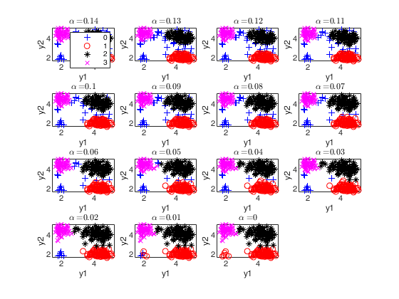
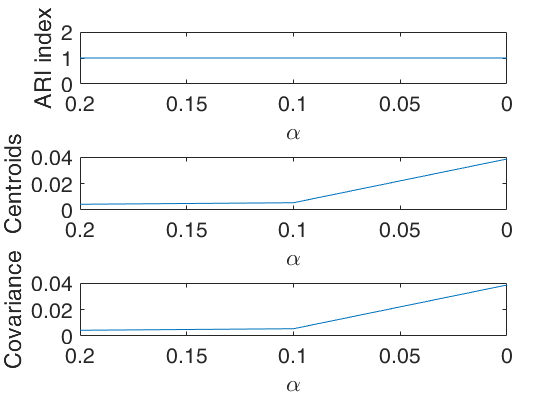
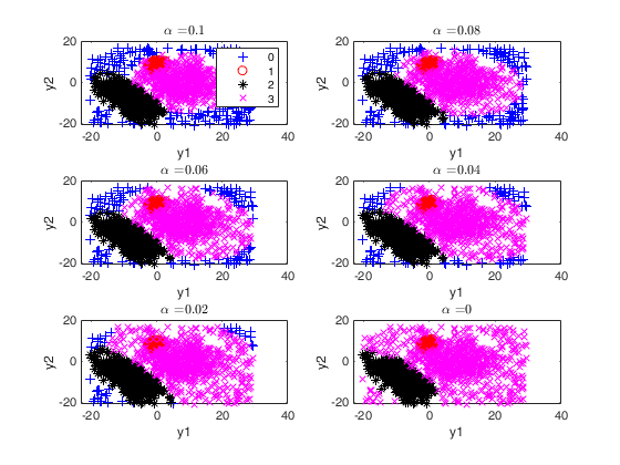
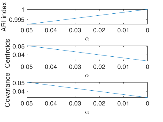
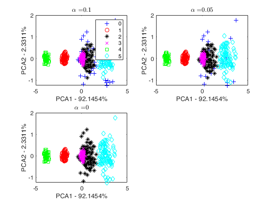
Case 1: plots option used as scalar.
- If plots=0, plots are not generated.
- If plots=1 (default), two plots are shown on the screen.
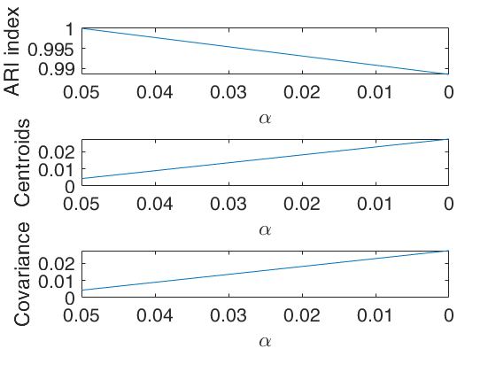
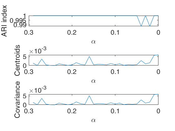
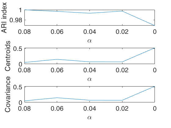
The first plot ("monitor plot") shows three panels
monitoring between two consecutive values of alpha the
change in classification using ARI index (top panel), the
change in centroids using squared euclidean distances
(central panel), the change in covariance matrices using
squared euclidean distance (bottom panel).
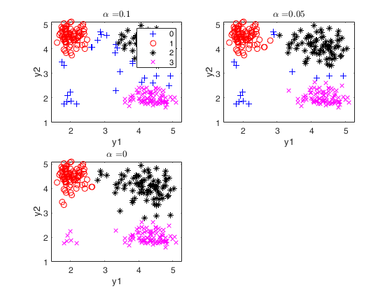
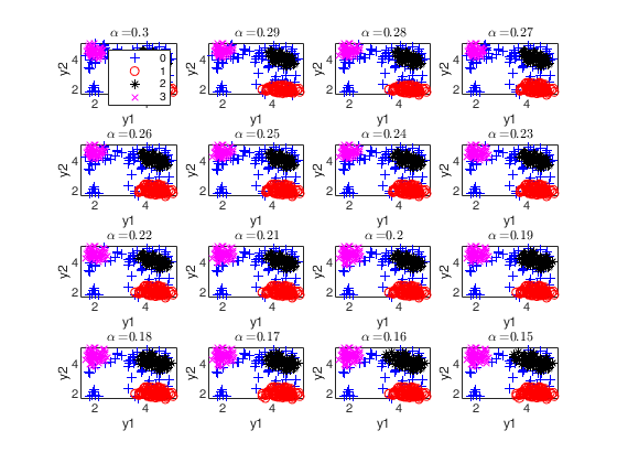
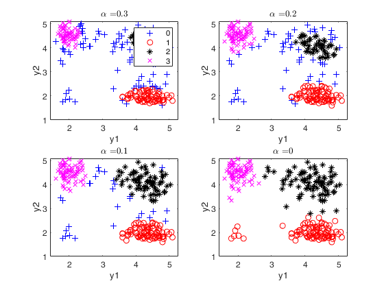
The second plot ("gscatter plot") shows a series of
subplots which monitor the classification for each value
of alpha. In order to make sure that consistent labels
are used for the groups, between two consecutive values
of alpha, we assign label r to a group if this group
shows the smallest distance with group r for the previous
value of alpha. The type of plot which is used to monitor
the stability of the classification depends on the value
of v.
* for v=1, we use histograms of the univariate data
(function histFS is called).
* for v=2, we use the scatter plot of the two
variables (function gscatter is called).
* for v>2, we use the scatter plot of the first two
principal components (function gscatter is called and
we show on the axes titles the percentage of variance
explained by the first two principal components).
Case 2: plots option used as struct.
If plots is a structure it may contain the following fields:
| Value |
Description |
name |
cell array of strings which enables to
specify which plot to display. plots.name = {'gscatter'}
produces a figure with a series of subplots which show the
classification for each value of alpha. plots.name = {'monitor'}
shows a figure with 3 panels which monitor between two
consecutive values of alpha the change in classification
using ARI index (top panel), the change in centroids
using squared euclidean distances (central panel), the
change in covariance matrices using squared euclidean
distance (bottom panel). If this field is
not specified plots.name={'gscatter' 'monitor'} and
both figures will be shown.
|
alphasel |
numeric vector which speciies for which
values of alpha it is possible to see the classification.
For example if plots.alphasel =[ 0.05 0.02], the
classification will be shown just for alpha=0.05 and
alpha=0.02; If this field is
not specified plots.alphasel=alpha and therefore the
classification is shown for each value of alpha.
|
ylimy |
2D array of size 3-by 2 which specifies the
lower and upper limits for the monitoring plots. The
first row refers the ARI index (top panel), the second
row refers to the the change in centroids using squared
euclidean distances (central panel), the third row is
associated with the change in covariance matrices using
squared euclidean distance (bottom panel).
|
Example: 'plots', 1
Data Types: single | double | struct
Scalar which controls whether to display or not messages
on the screen.
If msg=0 nothing is displayed on the screen.
If msg=1 (default) messages are displayed
on the screen about estimated time to compute the estimator
or the number of subsets in which there was no convergence.
If msg=2 detailed messages are displayed. For example the
information at iteration level.
Example: 'msg',1
Data Types: single | double
If nocheck is equal to 1 no check is performed on
matrix Y.
As default nocheck=0.
Example: 'nocheck',1
Data Types: single | double
If startv1 is 1 then initial centroids and covariance
matrices are based on (v+1) observations randomly chosen,
else each centroid is initialized taking a random row of
input data matrix and covariance matrices are initialized
with identity matrices. The default value of startv1 is 1.
Remark 1 - in order to start with a routine which is in the
required parameter space, eigenvalue restrictions are
immediately applied.
Remark 2 - option startv1 is used just if nsamp is a scalar
(see for more details the help associated with nsamp).
Example: 'startv1',1
Data Types: single | double
Matrix with size k-by-size(nsamp,1) containing the
random numbers which are used to initialize the
proportions of the groups. This option is effective just
if nsamp is a matrix which contains pre-extracted
subsamples. The purpose of this option is to enable to
user to replicate the results in case routine tclust is
called using a parfor instruction (as it happens for
example in routine tclustIC, where tclust is called through a
parfor for different values of the restriction factor).
The default value of RandNumbForNini is empty that is
random numbers from uniform are used.
Example: 'RandNumbForNini',''
Data Types: single | double
The type of restriction to
be applied on the cluster scatter
matrices. Valid values are 'eigen' (default), or 'deter'.
eigen implies restriction on the eigenvalues while deter
implies restriction on the determinants.
Example: 'restrtype','deter'
Data Types: char
This options only works
is 'restrtype' is 'deter'.
When restrtype is deter the default value of the "shape"
constraint (as defined below) applied to each group is fixed to
$c_{shape}=10^{10}$, to ensure the procedure is (virtually)
affine equivariant. In other words, the decomposition or the
$j$-th scatter matrix $\Sigma_j$ is
\[
\Sigma_j=\lambda_j^{1/v} \Omega_j \Gamma_j \Omega_j'
\]
where $\Omega_j$ is an orthogonal matrix of eigenvectors, $\Gamma_j$ is a
diagonal matrix with $|\Gamma_j|=1$ and with elements
$\{\gamma_{j1},...,\gamma_{jv}\}$ in its diagonal (proportional to
the eigenvalues of the $\Sigma_j$ matrix) and
$|\Sigma_j|=\lambda_j$. The $\Gamma_j$ matrices are commonly
known as "shape" matrices, because they determine the shape of the
fitted cluster components. The following $k$
constraints are then imposed on the shape matrices:
\[
\frac{\max_{l=1,...,v} \gamma_{jl}}{\min_{l=1,...,v} \gamma_{jl}}\leq
c_{shape}, \text{ for } j=1,...,k,
\]
In particular, if we are ideally searching for spherical
clusters it is necessary to set $c_{shape}=1$. Models with
variable volume and spherical clusters are handled with
'restrtype' 'deter', $1<restrfactor<\infty$ and $cshape=1$.
The $restrfactor=cshape=1$ case yields a very constrained
parametrization because it implies spherical clusters with
equal volumes.
Example: 'cshape',10
Data Types: single | double
For example if
UnitsSameGroup=[20 26], means that group which contains
unit 20 is always labelled with number 1. Similarly,
the group which contains unit 26 is always labelled
with number 2, (unless it is found that unit 26 already
belongs to group 1). In general, group which contains
unit UnitsSameGroup(r) where r=2, ...length(kk)-1 is
labelled with number r (unless it is found that unit
UnitsSameGroup(r) has already been assigned to groups
1, 2, ..., r-1).
Example: 'UnitsSameGroup',[20 34]
Data Types: integer vector
If
numpool is not defined, then it is set equal to the
number of physical cores in the computer.
Example: 'numpool',4
Data Types: integer vector
Indicated if the open pool
must be closed or not. It is useful to leave it open if
there are subsequent parallel sessions to execute, so
that to save the time required to open a new pool.
Example: 'cleanpool',true
Data Types: integer | logical
For some
specific case (e.g. translating to Python) this option
should be set to false.
Example: 'DfMmex',true
Data Types: integer | logical
 Monitoring using geyser data (all default options).