
|
tclustregeda |
tkmeans |
 |
tclustregIC
tclustregIC computes tclustreg for different number of groups k and restriction factors c
Description
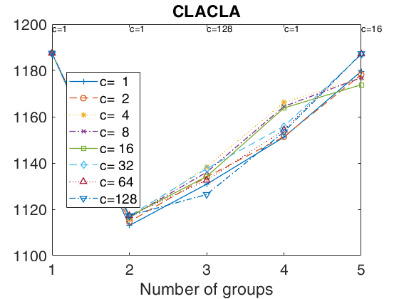
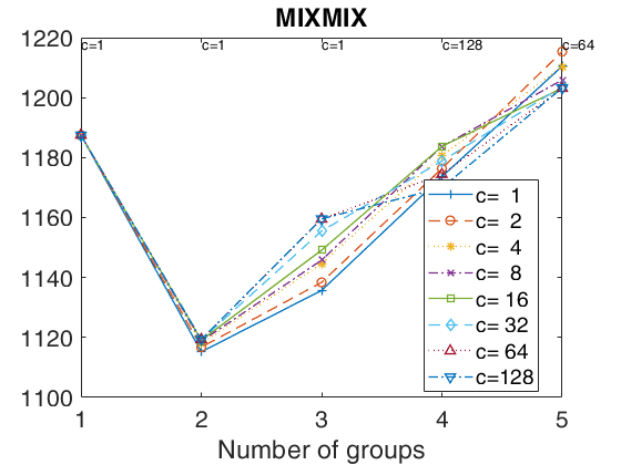
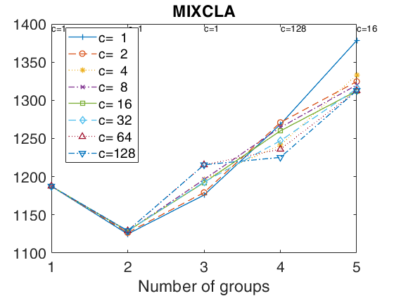
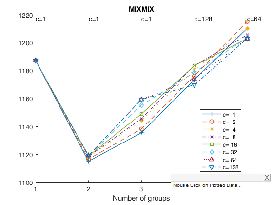
tclustregIC (where the last two letters stand for 'Information Criterion') computes the values of BIC (MIXMIX), ICL (MIXCLA) or CLA (CLACLA), for different values of k (number of groups) and different values of c (restriction factor for the variances of the residuals), for a prespecified level of trimming. If Parallel Computing toolbox is installed, parfor is used to compute tclustreg for different values of c. In order to minimize randomness, given k, the same subsets are used for each value of c.
tclustregIC of 'X data' with the handle 'h' option.out
=tclustregIC(y,
X,
Name, Value)
Examples
 tclustregIC of 'X data' with all default arguments.
tclustregIC of 'X data' with all default arguments.The X data have been introduced by Gordaliza, Garcia-Escudero & Mayo-Iscar (2013).
% The dataset presents two parallel components without contamination.
X  = load('X.txt');
y1 = X(:,end);
X1 = X(:,1:end-1);
out = tclustregIC(y1,X1,'plots',1);
tclustICplot(out,'whichIC','MIXMIX');
k=1
k=2
k=3
k=4
k=5
The labels of c in the top part of the plot denote the values of c for which IC is minimum
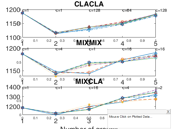
tclustregIC of 'X data' with the handle 'h' option.
tclustregIC of 'X data' with the handle 'h' option.The IC plot is copied into a subplot.
X  = load('X.txt');
y1 = X(:,end);
X1 = X(:,1:end-1);
h1   = subplot(3,1,1);
h2   = subplot(3,1,2);
h3   = subplot(3,1,3);
out = tclustregIC(y1,X1,'whichIC','CLACLA','plots',1,'h',h1);
out = tclustregIC(y1,X1,'whichIC','MIXMIX','plots',1,'h',h2);
out = tclustregIC(y1,X1,'whichIC','MIXCLA','plots',1,'h',h3);
k=1
k=2
k=3
k=4
k=5
The labels of c in the top part of the plot denote the values of c for which IC is minimum
k=1
k=2
k=3
k=4
k=5
The labels of c in the top part of the plot denote the values of c for which IC is minimum
k=1
k=2
k=3
k=4
k=5
The labels of c in the top part of the plot denote the values of c for which IC is minimum
Related Examples
tclustregIC using CWM model.
Generate mixture of regression using MixSimReg, with an average overlapping at centroids = 0.01. Use all default options.
rng(372,'twister');
p=3;
k=2;
Q=MixSimreg(k,p,'BarOmega',0.001);
n=500;
[y,X,id]=simdatasetreg(n,Q.Pi,Q.Beta,Q.S,Q.Xdistrib);
yXplot(y,X,id);
% run tclustreg with alphaX=1 that is using CWM.
out = tclustregIC(y,X(:,2:end),'alphaLik',0.0,'alphaX',1);
close all
tclustICplot(out,'whichIC','CLACLA')
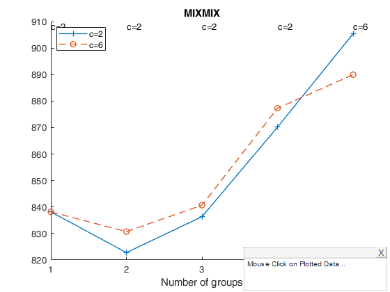
tclustregIC with simulated data with 4 groups.
tclustregIC with simulated data with 4 groups.Generate mixture of regression using MixSimReg, with an average overlapping at centroids =0.001.
rng(372,'twister');
p=3;
k=4;
Q=MixSimreg(k,p,'BarOmega',0.001);
n=200;
[y,X,id]=simdatasetreg(n,Q.Pi,Q.Beta,Q.S,Q.Xdistrib);
yXplot(y,X,id);
% Just consider two values for the restriction factor
out = tclustregIC(y,X(:,2:end),'alphaX',1,'cc',[2 6]);
close all
tclustICplot(out,'whichIC','MIXMIX')
k=1
k=2
k=3
k=4
k=5
tclustregIC with values of the restriction factor and number of groups supplied by the user.
Generate mixture of regression using MixSimReg, with an average overlapping at centroids =0.001.
rng(372,'twister');
p=3;
k=4;
Q=MixSimreg(k,p,'BarOmega',0.001);
n=200;
[y,X,id]=simdatasetreg(n,Q.Pi,Q.Beta,Q.S,Q.Xdistrib);
yXplot(y,X,id);
% Just consider two values for the restriction factor
out = tclustregIC(y,X(:,2:end),'alphaX',1,'cc',[2 6],'kk',3:6);
tclustICplot(out,'whichIC','MIXMIX')
Example of the use of CWM model with constraints on cov(X)
rng(191372,'twister');
p=3;
k=4;
Q=MixSimreg(k,p,'BarOmega',0.
rng(191372,'twister');
p=3;
k=4;
Q=MixSimreg(k,p,'BarOmega',0.001);
n=200;
[y,X,id]=simdatasetreg(n,Q.Pi,Q.Beta,Q.S,Q.Xdistrib);
yXplot(y,X,id);
% CWM with no contrainst on cov(X)
out = tclustregIC(y,X(:,2:end),'alphaX',1,'ccSigmaX',10^10);
tclustICplot(out,'whichIC','MIXMIX')
tclustregIC of fishery2003 with or without intercept.
clear all; close all;
rng(123)
intercept = 0;
load Fishery2003.mat;
X = Fishery2003{:,2};
X = X + 10^(-5) * abs(randn(size(X)));
y = Fishery2003{:,3};
y = y + 10^(-5) * abs(randn(size(y)));
id = Fishery2003{:,1};
% yXplot(yid,Xid);
% Use tclustregIC to monitor the effect of k and c, for alpha reasonably fixed
alpha = 0.01;
kvec  = 1:1:4;
cvec  = [1,2,4,8];
outIC = tclustregIC(y,X,'whichIC','CLACLA','kk',kvec,'cc',cvec,'alphaLik',alpha,'intercept',intercept,'plots',0);
% Extracts a set of best relevant solutions ...
[outICsol] = tclustICsol(outIC,'whichIC','CLACLA','plots',0,'NumberOfBestSolutions',5,'ThreshRandIndex',0.7);
% ... and visualise them with the carbike plot, which highlights the most
% relevant one in intuitive way.
[hcb,areas] = carbikeplot(outICsol,'SpuriousSolutions',false);
% Use the information extracted by tclustICsol to identify the best
% solution.
[truesol,~]  = ismember(outICsol.CLACLAbs(:,end),'true');
truesoli     = find(truesol);
[amax,iamax] = max(areas(truesoli,2));
if numel(truesoli) > 0
if amax>0
% take the true solution with larger area
kopt = outICsol.CLACLAbs{truesoli(iamax),1};  % optimal number of groups
copt = outICsol.CLACLAbs{truesoli(iamax),2};  % optimal nrestriction factor
else
% if areas are all zero, take the true solution with larger k
kopt = outICsol.CLACLAbs{truesoli(1),1};
copt = outICsol.CLACLAbs{truesoli(1),2};
end
else
% if there are no true solutions, take the one with larger k
kopt = outICsol.CLACLAbs{truesol(1),1};
copt = outICsol.CLACLAbs{truesol(1),2};
end
% Finally, use tclustregeda to monitor alpha, with k and c estimated by tclustregIC
alphaLikvec   = 0.05:-0.01:0;
outEDA        = tclustregeda(y,X,kopt,copt,alphaLikvec,0,'intercept',intercept,'plots',0);
% retrieve the optimal alpha
[ARImax]   = max(outEDA.Amon(:,2));
iARImax    = find(outEDA.Amon(:,2) == ARImax);
alphaopt   = outEDA.Amon(iARImax(end),1);
% final clustering % with the parameters sugggested by the monitoring
outTCLUST    = tclustreg(y,X,kopt,copt,alphaopt,0,'intercept',intercept,'plots',1);
idxTCLUST    = outTCLUST.idx;
Input Arguments
y — Response variable.
Vector.
A vector with n elements that contains the response variable.
y can be either a row or a column vector.
Data Types: single|double
X — Explanatory variables (also called 'regressors').
Matrix.
Data matrix of dimension . Rows of X represent observations, and columns represent variables. Missing values (NaN's) and infinite values (Inf's) are allowed, since observations (rows) with missing or infinite values will automatically be excluded from the computations.
Data Types: single|double
Name-Value Pair Arguments
Specify optional comma-separated pairs of Name,Value arguments.
Name is the argument name and Value
is the corresponding value. Name must appear
inside single quotes (' ').
You can specify several name and value pair arguments in any order as
Name1,Value1,...,NameN,ValueN.
 'alphaLik',0.1
, 'alphaX',1
, 'intercept',1
, 'cc',[1 2 4 8 128]
, 'ccsigmaX',10
, 'kk',1:4
, 'whichIC','ALL'
, 'nsamp',1000
, 'RandNumbForNini',''
, 'refsteps',10
, 'reftol',1e-05
, 'equalweights',true
, 'startv1',1
, 'plots',1
,'h',h1 where h1=subplot(2,1,1)
, 'numpool',4
, 'cleanpool',1
, 'msg',1
, 'nocheck',10
, 'Ysave',1
, 'UnitsSameGroup',[12 20]
, 'we',[0.2 0.2 0.2 0.2 0.2]
, 'commonslope',true
alphaLik
—Trimming level.scalar.
alphaLik is a value between 0 and 0.5 or an integer specifying the number of observations which have to be trimmed. If alphaLik=0 there is no trimming. More in detail, if 0<alphaLik<1 clustering is based on h=fix(n*(1-alphaLik)) observations.
Else if alphaLik is an integer greater than 1 clustering is based on h=n-floor(alphaLik). More in detail, likelihood contributions are sorted and the units associated with the smallest n-h contributions are trimmed.
The default value of alphaLik is 0 that is all the units are considered.
Example: 'alphaLik',0.1
Data Types: single | double
alphaX
—Second-level trimming or constrained weighted model for X.scalar.
alphaX is a value in the interval [0 1].
- If alphaX=0 there is no second-level trimming.
- If alphaX is in the interval [0 0.5] it indicates the fixed proportion of units subject to second level trimming.
In this case alphaX is usually smaller than alphaLik.
For further details see Garcia-Escudero et. al. (2010).
- If alphaX is in the interval (0.5 1), it indicates a Bonferronized confidence level to be used to identify the units subject to second level trimming. In this case the proportion of units subject to second level trimming is not fixed a priori, but is determined adaptively.
For further details see Torti et al. (2018).
- If alphaX=1, constrained weighted model for X is assumed (Gershenfeld, 1997). The CWM estimator is able to take into account different distributions for the explanatory variables across groups, so overcoming an intrinsic limitation of mixtures of regression, because they are implicitly assumed equally distributed. Note that if alphaX=1 it is also possible to apply, using input option ccsigmaX, constraints on the cov matrices of the explanatory variables.
For further details about CWM see Garcia-Escudero et al.
(2017) or Torti et al. (2018).
Example: 'alphaX',1
Data Types: single | double
intercept
—Indicator for constant term.scalar.
If 1, a model with constant term will be fitted (default), else no constant term will be included.
Example: 'intercept',1
Data Types: double
cc
—values of restriction factor for residual variances.vector.
A vector specifying the values of the restriction factor which have to be considered for the variances of the residuals of the regression lines.
The default value of cc is [1 2 4 8 16 32 64 128]
Example: 'cc',[1 2 4 8 128]
Data Types: double
ccSigmaX
—values of restriction factor for cov matrix of explanatory variables.scalar.
A scalar specifying the value of the restriction factor which has to be considered for the covariance matrices of the explanatory variables.
The default value of ccsigmaX is 12. Note that this option is used just if input option alphaX=1, that is if constrained weighted model (CWM) for X is assumed.
Example: 'ccsigmaX',10
Data Types: double
kk
—number of mixture components.integer vector.
Integer vector specifying the number of mixture components (clusters) for which the BIC is to be calculated.
Vector. The default value of kk is 1:5.
Example: 'kk',1:4
Data Types: int16 | int32 | single | double
whichIC
—type of information criterion.character.
Character which specifies which information criteria must be computed for each k (number of groups) and each value of the restriction factor (c).
Possible values for whichIC are: 'MIXMIX' = a mixture model is fitted and to compute the information criterion the mixture likelihood is used. This option corresponds to the use of the Bayesian Information criterion (BIC). In output structure out just the matrix out.MIXMIX is given.
'MIXCLA' = a mixture model is fitted but to compute the information criterion the classification likelihood is used. This option corresponds to the use of the Integrated Complete Likelihood (ICL). In output structure out just the matrix out.MIXCLA is given.
'CLACLA' = everything is based on the classification likelihood. This information criterion will be called CLA. In output structure out just the matrix out.CLACLA is given.
'ALL' = both classification and mixture likelihood are used.
In this case all the three information criteria CLA, ICL and BIC are computed. In output structure out all the three matrices out.MIXMIX and out.MIXCLA and out.CLACLA are given.
Example: 'whichIC','ALL'
Data Types: character
nsamp
—number of subsamples to extract.scalar | matrix.
If nsamp is a scalar it contains the number of subsamples which will be extracted. If nsamp=0 all subsets will be extracted.
Remark - if the number of all possible subset is <300 the default is to extract all subsets, otherwise just 300.
- If nsamp is a matrix it contains in the rows the indexes of the subsets which have to be extracted. nsamp in this case can be conveniently generated by function subsets.
nsamp can have k columns or k*(v+1) columns. If nsamp has k columns the k initial centroids each iteration i are given by X(nsamp(i,:),:) and the covariance matrices are equal to the identity.
- If nsamp has k*(v+1) columns the initial centroids and covariance matrices in iteration i are computed as follows X1=X(nsamp(i,:),:) mean(X1(1:v+1,:)) contains the initial centroid for group 1 cov(X1(1:v+1,:)) contains the initial cov matrix for group 1 1 mean(X1(v+2:2*v+2,:)) contains the initial centroid for group 2 cov((v+2:2*v+2,:)) contains the initial cov matrix for group 2 1 ...
mean(X1((k-1)*v+1:k*(v+1))) contains the initial centroids for group k cov(X1((k-1)*v+1:k*(v+1))) contains the initial cov matrix for group k REMARK - if nsamp is not a scalar option option below startv1 is ignored. More precisely if nsamp has k columns startv1=0 elseif nsamp has k*(v+1) columns option startv1=1.
Example: 'nsamp',1000
Data Types: double
RandNumbForNini
—Pre-extracted random numbers to initialize proportions.matrix.
Matrix with size k-by-size(nsamp,1) containing the random numbers which are used to initialize the proportions of the groups. This option is effective just if nsamp is a matrix which contains pre-extracted subsamples and k is a scalat. The purpose of this option is to enable the user to replicate the results.
The default value of RandNumbForNini is empty, that is random numbers from uniform are used.
Example: 'RandNumbForNini',''
Data Types: single | double
refsteps
—Number of refining iterations.scalar.
Number of refining iterations in subsample. Default is 15. refsteps = 0 means "raw-subsampling" without iterations.
Example: 'refsteps',10
Data Types: single | double
reftol
—scalar.default value of tolerance for the refining steps.
The default value is 1e-14;
Example: 'reftol',1e-05
Data Types: single | double
equalweights
—cluster weights in the concentration and assignment steps.logical.
A logical value specifying whether cluster weights shall be considered in the concentration, assignment steps and computation of the likelihood. Default value false.
Example: 'equalweights',true
Data Types: Logical
startv1
—how to initialize centroids and cov matrices.scalar.
If startv1 is 1 then initial centroids and and covariance matrices are based on (v+1) observations randomly chosen, else each centroid is initialized taking a random row of input data matrix and covariance matrices are initialized with identity matrices.
Remark 1- in order to start with a routine which is in the required parameter space, eigenvalue restrictions are immediately applied. The default value of startv1 is 1.
Remark 2 - option startv1 is used just if nsamp is a scalar (see for more details the help associated with nsamp).
Example: 'startv1',1
Data Types: single | double
plots
—Plot on the screen.scalar.
If plots = 1, a plot of the BIC (MIXMIX), ICL (MIXCLA)curve and CLACLA is shown on the screen. The plots which are shown depend on the input option 'whichIC'.
Example: 'plots',1
Data Types: single | double
h
—the axis handle of a figure where to send the IC plot.this can be used to host the IC plot in a subplot of a complex figure formed by different panels.
Example: 'h',h1 where h1=subplot(2,1,1)
Data Types: Axes object (supplied as a scalar)
numpool
—number of pools for parellel computing.scalar.
If numpool > 1, the routine automatically checks if the Parallel Computing Toolbox is installed and distributes the random starts over numpool parallel processes. If numpool <= 1, the random starts are run sequentially. By default, numpool is set equal to the number of physical cores available in the CPU (this choice may be inconvenient if other applications are running concurrently). The same happens if the numpool value chosen by the user exceeds the available number of cores. REMARK 1: up to R2013b, there was a limitation on the maximum number of cores that could be addressed by the parallel processing toolbox (8 and, more recently, 12). From R2014a, it is possible to run a local cluster of more than 12 workers.
REMARK 2: Unless you adjust the cluster profile, the default maximum number of workers is the same as the number of computational (physical) cores on the machine.
REMARK 3: In modern computers the number of logical cores is larger than the number of physical cores. By default, MATLAB is not using all logical cores because, normally, hyper-threading is enabled and some cores are reserved to this feature.
REMARK 4: It is because of Remarks 3 that we have chosen as default value for numpool the number of physical cores rather than the number of logical ones. The user can increase the number of parallel pool workers allocated to the multiple start monitoring by: - setting the NumWorkers option in the local cluster profile settings to the number of logical cores (Remark 2). To do so go on the menu "Home|Parallel|Manage Cluster Profile" and set the desired "Number of workers to start on your local machine".
- setting numpool to the desired number of workers;
Therefore, *if a parallel pool is not already open*, UserOption numpool (if set) overwrites the number of workers set in the local/current profile. Similarly, the number of workers in the local/current profile overwrites default value of 'numpool' obtained as feature('numCores') (i.e. the number of physical cores).
REMARK 5: the parallelization refers to the ...
Example: 'numpool',4
Data Types: double
cleanpool
—clean pool.scalar.
cleanpool is 1 if the parallel pool has to be cleaned after the execution of the routine. Otherwise it is 0. The default value of cleanpool is 0. Clearly this option has an effect just if previous option numpool is >
1.
Example: 'cleanpool',1
Data Types: single | double
msg
—Message on the screen.scalar.
Scalar which controls whether to display or not messages about code execution.
Example: 'msg',1
Data Types: single | double
nocheck
—Check input arguments.scalar.
If nocheck is equal to 1 no check is performed on matrix Y. As default nocheck=0.
Example: 'nocheck',10
Data Types: single | double
Ysave
—save input matrix.scalar.
Scalar that is set to 1 to request that the input vector y and input matrix X is saved into the output structure out. Default is 1, that is vector y and matrix X are saved inside output structure out.
Example: 'Ysave',1
Data Types: single | double
UnitsSameGroup
—Units with same labels.numeric vector.
List of the units which must (whenever possible) have the same label. For example if UnitsSameGroup=[20 26], it means that group which contains unit 20 is always labelled with number 1. Similarly, the group which contains unit 26 is always labelled with number 2, (unless it is found that unit 26 already belongs to group 1). In general, group which contains unit UnitsSameGroup(r) where r=2, ...length(kk)-1 is labelled with number r (unless it is found that unit UnitsSameGroup(r) has already been assigned to groups 1, 2, ..., r-1). The default value of UnitsSameGroup is '' that is consistent labels are not imposed.
Example: 'UnitsSameGroup',[12 20]
Data Types: single | double
we
—Vector of observation weights.vector.
A vector of size n-by-1 containing application-specific weights that the user needs to apply to each observation. Default value is a vector of ones.
Remark: The user should only give the input arguments that have to change their default value. The name of the input arguments needs to be followed by their value. The order of the input arguments is of no importance.
Example: 'we',[0.2 0.2 0.2 0.2 0.2]
Data Types: double
commonslope
—Impose constraint of common slope regression coefficients.boolean.
If commonslope is true, the groups are forced to have the same regression coefficients (apart from the intercepts).
The default value of commonslope is false;
Example: 'commonslope',true
Data Types: boolean
Output Arguments
out — description
Structure
Structure which contains the following fields:
| Value | Description |
|---|---|
CLACLA |
matrix of size 5-times-8 if kk and ccsigmay are not specififed else it is a matrix of size length(kk)-times length(cc) containinig the value of the penalized classification likelihood. This output is present only if 'whichIC' is 'CLACLA' or 'whichIC' is 'ALL'. |
CLACLAtable |
same output of CLACLA but in MATLAB table format (this field is present only if your MATLAB version is not<2013b). |
IDXCLA |
cell of size 5-times-8 if kk and cc are not specififed else it is a cell of size length(kk)-times length(cc). Each element of the cell is a vector of length n containinig the assignment of each unit using the classification model. This output is present only if 'whichIC' is 'CLACLA' or 'whichIC' is 'ALL'. |
MIXMIX |
matrix of size 5-times-8 if kk and cc are not specififed else it is a matrix of size length(kk)-times length(cc) containinig the value of the penalized mixture likelihood. This output is present only if 'whichIC' is 'MIXMIX' or 'whichIC' is 'ALL'. |
MIXMIXtable |
same output of MIXMIX but in MATLAB table format (this field is present only if your MATLAB version is not<2013b). |
MIXCLA |
matrix of size 5-times-8 if kk and cc are not specififed else it is a matrix of size length(kk)-times length(cc) containinig the value of the ICL. This output is present only if 'whichIC' is 'MIXCLA' or 'whichIC' is 'ALL'. |
MIXCLAtable |
same output of MIXCLA but in MATLAB table format (this field is present only if your MATLAB version is not<2013b). |
IDXMIX |
cell of size 5-times-8 if kk and cc are not specififed else it is a cell of size length(kk)-times length(cc). Each element of the cell is a vector of length n containinig the assignment of each unit using the mixture model. This output is present only if 'whichIC' is 'MIXMIX', 'MIXCLA' or 'ALL'. |
kk |
vector containing the values of k (number of components) which have been considered. This vector is equal to input optional argument kk if kk had been specified else it is equal to 1:5. |
cc |
vector containing the values of c (values of the restriction factor) which have been considered for the variance of the residuals. This vector is equal to input optional argument ccsigmay if ccsigmay had been specified else it is equal to [1, 2, 4, 8, 16, 32, 64, 128]. |
ccSigmaX |
vector containing the values of c (values of the restriction factor) which have been considered for the covariance matrices of the esplnatory variables. This vector is equal to input optional argument ccsigmaX if ccsigmaX had been specified and input option alphaX=1 otherwise it is equal to 12 if alphaX=1 and xxsigmaX has not been specified. Finally if input option alphaX is not equal 1 out.ccsigmaX is an empty value |
alpha |
scalar containing the trimming level which has been used in the likelidood (it stores the values of input alphaLik). |
alphaX |
scalar containing information about second-level trimming or constrained weighted model for X. |
X |
Original data matrix of explanatory variables. The field is present if option Ysave is set to 1. |
y |
Original vector containing the response The field is present if option Ysave is set to 1. |
References
Torti F., Perrotta D., Riani, M. and Cerioli A. (2019). Assessing Robust Methodologies for Clustering Linear Regression Data, "Advances in Data Analysis and Classification", Vol. 13, pp. 227–257, https://doi.org/10.1007/s11634-018-0331-4
See Also
|
|
tclustregeda |
tkmeans |
|
|
|
Functions |
|
• The developers of the toolbox • The forward search group • Terms of Use • Acknowledgments