twdrnd
TWDRND generates random variates from the Tweedie distribution.
Description
This function generates random numbers from a Tweedie distribution, with parameter space given by (\alpha,\theta,\gamma) = \Big\{\; ]-\inf , 0[ \;\times\; ]0,\inf[ \;\times\; ]0,\inf[ \;\Big\} \cup \Big\{\; ]0 , 1[ \;\times\; [0,\inf[ \;\times\; ]0,\inf[ \;\Big\}
The parameter space follows the Laplace transform formulation of Hougaard (1986) and Hougaard et al. (1997), The parameter \delta crucially determines the characteristics of the Tweedie distribution. The family includes the continuous normal, gamma and inverse gaussian distributions.
\delta = 0 is for the gaussian.
\delta = 1 is for the poisson.
\delta = 2 is for the gamma.
\delta = 3 is for the inverse gaussian.
Examples
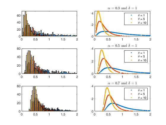
 Plots of pdf and histogram of generated data for some parameter choices.
Plots of pdf and histogram of generated data for some parameter choices.Parametrizations: alpha, theta, delta Hougaard (1986) and Hougaard et al. (1997).
% alpha, beta, gamma (Devroye (2009)).
% $\beta  = \theta \delta^{1/alpha}$.
% $\gamma = \delta^{1/alpha}$.
alpha = [0.3 , 0.5 , 0.7];
theta = [1 , 5 , 10] ;
delta = [1 , 1 , 1];
beta  = theta.*delta.^(1./alpha);
gamma = delta.^(1./alpha);
n= 500;
hf = figure; af = gca(hf);
for i=1:3
hs1 = subplot(3,2,2*i-1);
hs2 = subplot(3,2,2*i);
leg = [];
for j=1:3
% generate random data vector X
X    = twdrnd(alpha(i),theta(j),delta(i),n);
bins = round(n/(2*theta(j)));
histogram(hs1,X,bins); hold(hs1,'on');
% use X to make the pdf
pdf = twdpdf(X,alpha(i),theta(j),delta(i));
plot(hs2,X,pdf,'.'); hold(hs2,'on');
xlim([hs1,hs2],[0,2]);
% to be used in the legend
assignin('caller',['leg' num2str(j)],['\theta = ' num2str(theta(j))]);
end
title(['$\alpha = ' num2str(alpha(i)) ' \mbox{ and } \delta = ' num2str(delta(i)) '$'] , 'interpreter','latex');
legend(leg1,leg2,leg3);
end
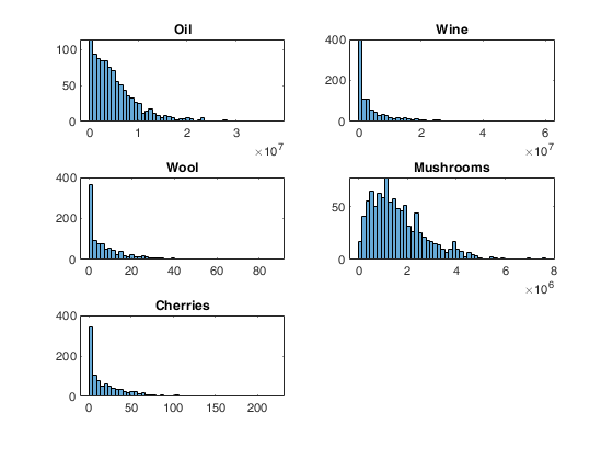
Examples from Barabesi et al (2016).
Examples from Barabesi et al (2016).
n = 1000;
pOil       = [-0.2697 , 0.291*10^(-6)  , 0.0282];
pWine      = [-0.0178 , 0.7802*10^(-7) , 0.3158];
pWool      = [-0.7380 , 0.145          , 0.2615];
pMushrooms = [-0.0936 , 1.27 *10^(-6)  , 0.6145];
pCherries  = [-0.3221 , 0.0324         , 0.2510];
param1 = pOil;          tit1 = 'Oil';
param2 = pWine;         tit2 = 'Wine';
param3 = pWool;         tit3 = 'Wool';
param4 = pMushrooms;    tit4 = 'Mushrooms';
param5 = pCherries;     tit5 = 'Cherries';
figure;
bins = round(n/20);
h1 = subplot(3,2,1);
al = param1(1) ; th = param1(2) ; de = param1(3) ;
t = twdrnd(al,th,de,n);
histogram(h1,t,bins);
title(h1,tit1);
h2 = subplot(3,2,2);
al = param2(1) ; th = param2(2) ; de = param2(3) ;
t = twdrnd(al,th,de,n);
histogram(h2,t,bins);
title(h2,tit2);
h3 = subplot(3,2,3);
al = param3(1) ; th = param3(2) ; de = param3(3) ;
t = twdrnd(al,th,de,n);
histogram(h3,t,bins);
title(h3,tit3);
h4 = subplot(3,2,4);
al = param4(1) ; th = param4(2) ; de = param4(3) ;
t = twdrnd(al,th,de,n);
histogram(h4,t,bins);
title(h4,tit4);
h5 = subplot(3,2,5);
al = param5(1) ; th = param5(2) ; de = param5(3) ;
t = twdrnd(al,th,de,n);
histogram(h5,t,bins);
title(h5,tit5);
Input Arguments
Output Arguments
More About
References
Tweedie, M. C. K. (1984), An index which distinguishes between some important exponential families, "in Statistics: Applications and New Directions, Proceedings of the Indian Statistical Institute Golden Jubilee International Conference (J.K. Ghosh and J. Roy, eds.), Indian Statistical Institute, Calcutta", pp. 579-604.
Jorgensen, B. (1987), Exponential dispersion models, "Journal of the Royal Statistical Society, Series B", Vol.49, pp. 127-162.
Hougaard, P. (1986), Survival models for heterogeneous populations derived from stable distributions, "Biometrika", Vol. 73, pp. 387-396.
Hougaard, P., Lee M.T. and Whitmore, G.A. (1997), Analysis of overdispersed count data by mixtures of Poisson variables and Poisson processes, "Biometrics", Vol. 53, pp. 1225-1238.
Dunn, P. K. and Smyth, G. K. (2005), Series Evaluation of Tweedie Exponential Dispersion Model Densities, "Statistics and Computing", Vol. 15, pp. 267–280.
Dunn, P. K. and Smyth, G. K. (2008), Series Evaluation of Tweedie Exponential Dispersion Model Densities by Fourier Inversion, "Statistics and Computing", Vol. 18, pp. 73–86.
Barabesi, L., Cerasa, A., Perrotta, D. and Cerioli, A. (2016), Modeling international trade data with the Tweedie distribution for anti-fraud and policy support, "European Journal of Operational Research", Vol. 248, pp. 1031-1043.