FSMedaeasy
FSMedaeasy is exactly equal to FSMeda but it is much less efficient
Description
Examples
 FSMeda with optional arguments (minimum Mahalanobis distance monitoring).
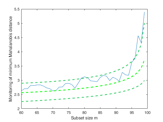
FSMeda with optional arguments (minimum Mahalanobis distance monitoring).Monitoring the evolution of minimum Mahalanobis distance.
n=100;
v=3;
m0=3;
Y=randn(n,v);
% Contaminated data
Ycont=Y;
Ycont(1:5,:)=Ycont(1:5,:)+3;
[fre]=unibiv(Y);
%create an initial subset with the 3 observations with the lowest
%Mahalanobis Distance
fre=sortrows(fre,4);
bs=fre(1:m0,1);
[out]=FSMedaeasy(Ycont,bs,'plots',1);
Warning: Matrix is close to singular or badly scaled. Results may be inaccurate.
RCOND =  1.641939e-16.
Related Examples
FSMeda with optional arguments (centroid position monitoring).
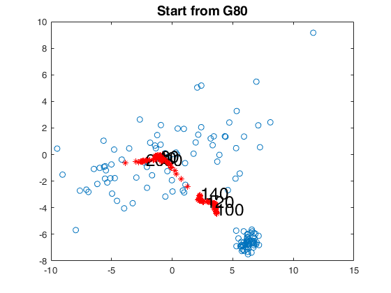
FSMeda with optional arguments (centroid position monitoring).Monitoring the minimum Mahalanobis distance and the centroid position.
% In this example the figures of minimum Mahalanobis distance are closed.
Y=load('sixty_eighty.txt');
G = 60*ones(140,1);
G(1:80)=80;
n = size(Y,1);
init = floor(n/2);
% start from G80
bs80 = [1,2,3];
[out80]=FSMedaeasy(Y,bs80,'plots',2,'init',init,'scaled',1);
close(findobj('tag','pl_mmd'));
title('Start from G80','Fontsize',14);
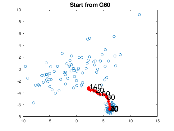
% start from G60
bs60 = [81,82,83];
[out60]=FSMedaeasy(Y,bs60,'plots',2,'init',init,'scaled',1);
close(findobj('tag','pl_mmd'));
title('Start from G60','Fontsize',14);
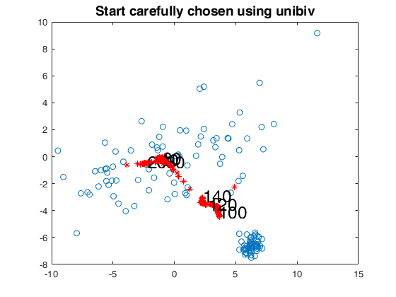
% start in an optimal way automatically
[fre]=unibiv(Y,'plots',0,'rf',0.5);
fre=sortrows(fre,4);
init=2;
bs=fre(1:init,1);
[out]=FSMedaeasy(Y,bs,'plots',2,'init',init,'scaled',1);
close(findobj('tag','pl_mmd'));
title('Start carefully chosen using unibiv','Fontsize',14);Warning: interchange greater than 10 when m=92 Number of units which entered=25 Attention : init1 should be larger than v. It is set to v+1. Warning: interchange greater than 10 when m=92 Number of units which entered=25
Example with the Swiss bank notes data.
Example with the Swiss bank notes data.
load('swiss_banknotes');
Y=swiss_banknotes{:,:};
[fre]=unibiv(Y);
%create an initial subset with the 3 observations with the lowest
%Mahalanobis Distance
fre=sortrows(fre,4);
m0=20;
bs=fre(1:m0,1);
[out]=FSMedaeasy(Y,bs,'plots',1,'init',30);
Input Arguments
Output Arguments
References
Atkinson, A.C., Riani, M. and Cerioli, A. (2004), "Exploring multivariate data with the forward search", Springer Verlag, New York.